Study of Otto Cycle using Matlab

Aim:

• To plot the pressure vs volume graph of an air standard Otto cycle using MATLAB
• To find the efficiency of air standard Otto cycle.

Notations used:

• `v_s`-Swept volume
• `v_c`-Clearance volume
• `r_c`-Compression ratio
• `theta`-Crank angle

Formulas used:

• Crank radius `a=(stroke)/2`.
• Crank pin radius `R=(stroke)/a`
• Clearance volume `v_c=v_s/(r_c-1)`
• Swept volume `v_s=pi/4("bore")^2(stroke)`
• Volume inside cylinder `v=v_c[1+1/2(r_c-1)(R+1-costheta-(R^2-sin^2theta)^0.5]``
• Efficiency `eta=1-1/r_c^(gamma-1)`

Inputs assumed:

• Initially we assume pressure(p1) and temperature(t1) of air entering the cylinder.
• We also assume engine geometric parameters like bore,stroke length, connecting rod length.
• As the assumed working fluid is air we can take value of `gamma=1.4`.
• Also the temperature of working fluid after combustion is assumed as `t3=2500K`.

Evaluation of pressure and volume at each stage:

• Initial volume(v1) can be given by `v_1=v_s+v_c`.
• At state 2 volume(v2) is equal to clearance volume(`v_c`).
• Pressure at state 2 (p2) is calculated using `pv^gamma="constant"`as it is isentropic compression process.
• Volume at state 3 is same as volume at state 2 as process is constant volume heat addition process (`v_3=v_2`)
• As temperature at state 3 is assumed and known we can find pressure at 3 using ideal gas equation `(PV)/T="constant"`
• Volume at state 4 will be same as state 1 as process is constant volume heat rejection process `v_4=v_1`
• Pressure at state 4 can be calculated using `pv^gamma="constant"`as the process is isentropic expansion

Initial plotting of obtained points:

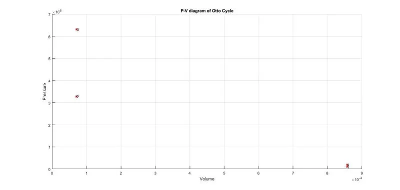
• Now, that we have obtained values of pressure and volume at each stage it can be plotted as

Volume in cylinder as function of crank angle:

• Now we cannot connect the points using straight line as the volume is not varying linearly with crank angle.
• So the volume variation with crank angle is given by relation `v=v_c[1+1/2(r_c-1)(R+1-costheta-(R^2-sin^2theta)^0.5]``
• We include this formula in seperate function and pass on the input arguments as crank start and crank end angles based on whether the process is compression or expansion.
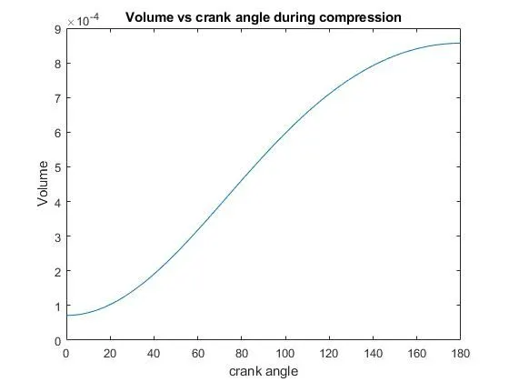
• We pass on input arguments as crank start angle=0 and crank end angle=180 for compression,and corresponding variation can be illustrated as:
• We pass input arguments as crank start angle=180 and crank end angle=0 for expansion.
• Based on the obtained output argument from function, we plot the graph accordingly.

Code:

% function to calculate volume as function of crank angle

function v= kinematics(crank_start,crank_end)
bore=0.1;
stroke=0.1;
r_c=12;
con_rod=0.15;

%crank pin radius calculation

a=stroke/2;
crank_radius=con_rod/a;

%calculation of swept and clearance volumes

v_s=pi/4*bore^2*stroke;
v_c=v_s/(r_c-1);
theta=linspace(crank_start,crank_end,100);

%calculation of volume variation with crank angle

term_1=0.5*(r_c-1);
term_2=crank_radius+1-cosd(theta);
term_3=sqrt(crank_radius^2-sind(theta).^2);
v=[1+term_1*(term_2-term_3)].*v_c;

end


% inputs or assumed values

p1=101325;
t1=500;
t3=2600;
gamma=1.4;
v1=v_s+v_c;

%Function call

v_compression=kinematics(0,180);
p_compression=p_1*(v1./v_compression).^gamma;
hold on
plot(v_compression,p_compression)

v2=v_c;

% Process 1-2 is isentropic compression so PV^gamma=constant

p2=p1*cr^gamma;
t2=p2*v2*t1/(p1*v1);

% Process 2-3 is constant volume heat addition

v3=v2;
p3=p2*t3/t2;

% Process 3-4 is isentropic compression so PV^gamma=constant

p4=p3*(1/cr)^gamma;

% Process 4-1 is constant volume heat rejection

v4=v1;


%function call

v_expansion=kinematics(180,0);
p_expansion=p3*(v3./v_expansion).^gamma;

%plotting the obtained pressure and volume for various crank angles

plot(v_expansion,p_expansion)
plot([v2,v3],[p2,p3])
plot([v1,v4],[p1,p4])
grid on
xlabel('Volume')
ylabel('Pressure')
title('P-V diagram of Otto Cycle')
text([v1,v2,v3,v4],[p1,p2,p3,p4],{'1','2','3','4'})

%Formula to calculate efficiency of the cycle

efficiency=[1-1/cr^(gamma-1)]*100

Results:

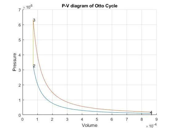
• Plot is obtained as:
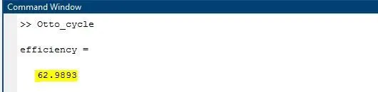
• Efficiency is calculated as: