Solving second order ODE's using MATLAB

Aim:

• To study the variation of velocity and displacement of vibrating body under damping.
• To find the natural and damped frequency of vibrating body.

Notations used:

• `c`-Damping coefficeint in`(Ns)/m`.
• `m`- Mass in kg.
• `k`-Stiffness of spring in `N/m`.
• `x`-Displacement of the body in m.

Background theory:

• Motion of simple pendulum can be consodered to be in SHM, as the acceleration of body is diectly proprtional to its displacement.
• The governing equation of motion of pendulum can be given by:`(d^2x)/dt^2+c/m(dx/dt)+k/mx=0`.
• Solving this second order ODE analytically involves using RK-4th order method, which is quite laborious due to large number of iterations.
• So for this reason analysis is done using MATLAB.

Usage of ODE45 in MATLAB:

• The function ode 45 takes 3 inputs, namely the function to be integrated,time span, and the initial conditions of the considered mechanical system.
• The time span would be the integration limits. This can be provided as a vector of 2 values, the initial and final time or with a spacing using the linspace function. The solver will choose a step size that is most suitable for the solution to obtain solution in the most optimal time possible. The initial condition would be the value of the function at t=0.
• ODE 45 can solve only first order differential equations, so we need to convert our problem into first using suitable assumptions.

Assumptions or Input values:

• `c`=`0.05(Ns)/m`
• `m= 0.1kg`
• `k= 1N/m`
• Initial displacement= 0m
• Initial velocity=`5m/s`
• Time period under consideration=10s.

Code:

% initial displacement=0; initial velocity=5m/s
x_0=[0;5];

% time under consideration with step size of 500
tspan=linspace(0,15,500);

% inputs
c=0.05;     %damping coefficeint in Ns/m
k=1;        %length of simple pendulum in m
m=0.1;      % mass of oscillating body in kg

% function call describing time duration and initial conditions
[t,results]=ode45(@(t,x) myode(t,x,c,k,m),tspan,x_0);
% results matrix contains displacement and velocity details of the body


% plotting displacement vs time
plot (t,results(:,1))
xlabel('time(s)')
ylabel('Displacement(m)/velocity(m/s)')
hold on

% plotting velocity vs time
plot(t,results(:,2))
legend('Displacement','Velocity')

%calculation of natural frequency
w_n=sqrt(k/m);

%damping ratio
e=c/2*sqrt(k*m);

%damped frequency
w_d=[sqrt(1-e^2)]*w_n;
fprintf('Natural frequency is %f\n', w_n)
fprintf('Damped frequency is %f\n', w_d)


% function definition to convert seond order differential to first order

function[dx_dt]=myode(t,x,c,k,m)
x1=x(1);        
x2=x(2);
dx1_dt=x2;        % converting to first order differential by assuming dx1_dt=x2
dx2_dt=-(c/m)*x2-(k/m)*(x1);
dx_dt=[dx1_dt;dx2_dt];  % first order ODE matrix to be integrated in ODE45 function
end

Results:

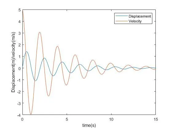
• We obtain the plot as shown below , where displacement and velocity of body decreases gradually due to damping.

• Natural frequency and damped frequency is obtained as: