Week 6 - Understanding the stability analysis in linear systems

6. Understanding the stability analysis in linear systems

OBJECTIVE

1. Solve the system of matrices using Jacobi, Gauss-seidel, and SOR methods.
2. Compute the Iteration Matrix for the iterative methods by suitable matrix decomposition techniques taught in the lectures.
3. Calculate the Eigenvalues of the Iteration matrix.
4. Calculate the Spectral radius of the Iteration matrix.
5. Explain Diagonal dominance and its importance.

GIVEN

Consider the following system of matrices.

• Coefficient Matrix, A=[5 1 2 ; -3 9 4; 1 2 -7]
• Solution Matrix, X=[x1;x2;x3]
• Residual Matrix, B=[10 -14 33]

THEORY

Eigenvalues

• Eigenvalues are a unique set of scalars associated with a linear system of equations.
• They are also known as characteristic roots, characteristic values of a matrix
• The determination of the eigenvalues of a system is significant in engineering and arises in such typical applications as stability analysis, the physics of rotating bodies, and small oscillations of vibrating systems

• Let A be a linear transformation represented by a matrix A. If there is a vector X∈Rn">X∈Rn�∈�� such that

AX=λX">AX=λX��=��

for some scalar λ">λ�, then λ">λ� is called the eigenvalue of A with the corresponding (right) eigenvector X.

Spectral Radius

• The largest absolute value or complex modulus of its eigenvalues.
• If the value of the spectral radius is high, the solution might not converge.

Diagonal Dominance

• The matrix is said to be strictly diagonally dominant if and only if the magnitude of the diagonal element in a row is greater than the sum of the magnitudes of other elements in the row.
• Boundedness is the condition for convergence. The spectral radius value of less than 1 and the diagonally dominant matrix imply that the solution at all the nodes is bounded (converged).

Jacobi Method

• XNEW=D-1⋅(B-((L+U)⋅XOLD))">XNEW=D−1⋅(B−((L+U)⋅XOLD))����=�-1⋅(�-((�+�)⋅����))
• Iteration Matrix

T=-D-1⋅(L+U)">T=−D−1⋅(L+U)�=-�-1⋅(�+�)

• Diagonal matrix=D

  Lower triangular matrix=L

  Upper triangular martrix=U

  Identity matrix = I

Gauss-Seidel Method

• XNEW=(L+D)-1⋅(B-(U⋅XOLD))">XNEW=(L+D)−1⋅(B−(U⋅XOLD))����=(�+�)-1⋅(�-(�⋅����))
• Iteration Matrix

T=-(L+Dm)-1⋅U">T=−(L+Dm)−1⋅U�=-(�+��)-1⋅�

SOR Method

• XNEW=ω⋅(L+D)-1⋅B-(I-ω⋅((L+D)-1⋅U+I))⋅XOLD">XNEW=ω⋅(L+D)−1⋅B−(I−ω⋅((L+D)−1⋅U+I))⋅XOLD����=�⋅(�+�)-1⋅�-(�-�⋅((�+�)-1⋅�+�))⋅����
• Iteration Matrix

T=I-ω⋅((L+D)-1⋅U+I))">T=I−ω⋅((L+D)−1⋅U+I))�=�-�⋅((�+�)-1⋅�+�))

MATLAB CODE

Main Program

clear
close all
clc

% Coefficient matrix
A=[5 1 2;-3 9 4;1 2 -7];
% Lower triangular matrix
L=[0 0 0;-3 0 0;1 2 0];
% Upper triangular matrix
U=[0 1 2;0 0 4;0 0 0];
% Diagonal matrix
D1=[5 0 0;0 9 0;0 0 -7];

% Residual Matrix
B=[10;-14;33];
% Identity matrix
I=[1 0 0; 0 1 0;0 0 1];

% omega
omega=1.25;

% Diagonal magnification
Dm=(1:1:10);
for i=1:length(Dm)
    D=D1*Dm(i);
    
    % iteration matrix for Jacobi
    T_jac=inv(D)*(-L-U);
    eigenvalue_jacobi=roots(poly(T_jac));
    spectral_radius_jacobi(i)=max(abs(real(eigenvalue_jacobi)));

    % calling jacobian function
    [jac_iter(i),X]=jacobi_linear(L,D,U,B);
   
    % iteration matrix for gauss-seidel method
    T_gs=-U*inv(L+D);
    eigenvalue_gs=roots(poly(T_gs));
    spectral_radius_gs(i)=max(abs(real(eigenvalue_gs)));
    % calling Gauss-seidel function
    [GS_iter(i),X]=gs_linear(L,D,U,B);
  
    % iteration matrix for successive over-relaxation method
    T_sor=inv(D+(omega*L))*(((1-omega)*D)-(U*omega));
    eigenvalue_sor=roots(poly(T_sor));
    spectral_radius_sor(i)=max(abs(real(eigenvalue_sor)));
    % calling SOR method function
    [SOR_iter(i),X]=sor_linear(L,D,U,B,omega);
    
end
    % Plotting graphs
    % Jacobi method
    figure(1)
    subplot(2,1,1)
    plot(Dm,spectral_radius_jacobi)
    grid on
    xlabel('Diagonal magnification')
    ylabel('Spectral radius')
    title('Jacobi Method')
    
    subplot(2,1,2)
    plot(spectral_radius_jacobi,jac_iter)
    grid on 
    xlabel('Spectral radius')
    ylabel('Number of Jacobi iterations')
    
    % GS Method
    figure(2)
    subplot(2,1,1)
    plot(Dm,spectral_radius_gs)
    grid on
    xlabel('Diagonal magnification')
    ylabel('Spectral radius')
    title('GS Method')
    
    subplot(2,1,2)
    plot(spectral_radius_gs,GS_iter)
    grid on 
    xlabel('Spectral radius')
    ylabel('Number of GS iterations')
    
    % SOR Method
    figure(3)
    subplot(2,1,1)
    plot(Dm,spectral_radius_sor)
    grid on
    xlabel('Diagonal magnification')
    ylabel('Spectral radius')
    title('SOR Method')
    
    subplot(2,1,2)
    plot(spectral_radius_sor,SOR_iter)
    grid on 
    xlabel('Spectral radius')
    ylabel('Number of SOR iterations')
    

Jacobi method Function

function [jac_iter,X]=jacobi_linear(L,D,U,B)
error=9e9;
tol=1e-4;
jac_iter=1;
Xold=[0;0;0];

    % jacobi iteration
    while(error>tol)
    X=inv(D)*B+(inv(D)*(-L-U)*Xold);
    
    error=max(abs(Xold-X));
    Xold=X;
    jac_iter=jac_iter+1;
    end
    
end

Gauss-Seidel Function

function [GS_iter,X]=gs_linear(L,D,U,B)
error=9e9;
tol=1e-4;
GS_iter=1;
Xold=[0;0;0];

    % Gauss Seidel Method
    while(error>tol)
    X=inv(L+D)*B+(inv(L+D)*(-U)*Xold);
    
    error=max(abs(Xold-X));
    Xold=X;
    GS_iter=GS_iter+1;
    end
    
end

SOR method Function

function [SOR_iter,X]=sor_linear(L,D,U,B,omega)
error=9e9;
tol=1e-4;
SOR_iter=1;
Xold=[0;0;0];
I=[1 0 0; 0 1 0;0 0 1];

    % SOR method
    while(error>tol)
    X=((1-omega)*Xold+(omega*((inv(D+L)*B)+inv(D+L)*(-U)*Xold)));
    
    error=max(abs(Xold-X));
    Xold=X;
    SOR_iter=SOR_iter+1;
    end
    
end

EXPLANATION

1. Using LDU decomposition, obtain the values of L, D, and U.
2. Assign the diagonal modification vector and apply it to the diagonal matrix.
3. Next, create a for loop for calculating eigenvalues and spectral radius.
4. Inside the loop, calculate the iteration matrix for all the iterative methods along with eigenvalues and spectral radius.
5. Now call the user-defined function to calculate the iterative solution.
6. The last step is to plot the required graphs (diagonal magnification and spectral radius) & (spectral radius and the number of iterations) to derive conclusions.

RESULTS

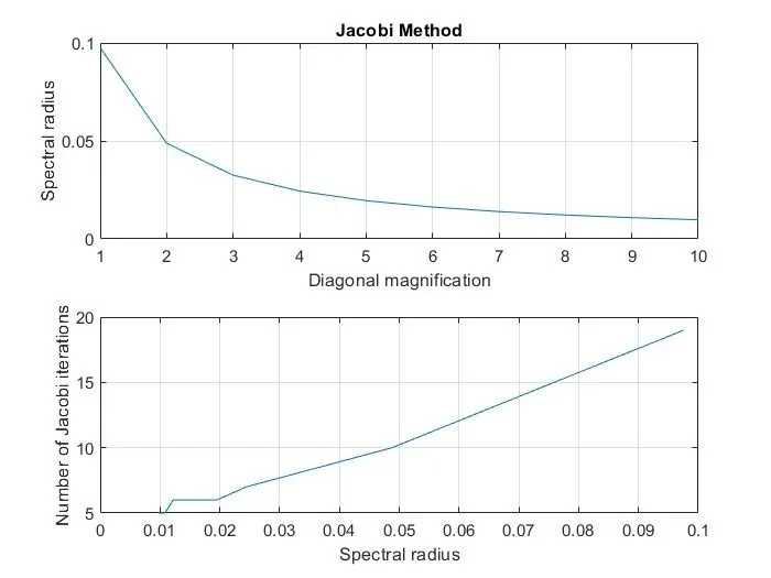
• Jacobi Method

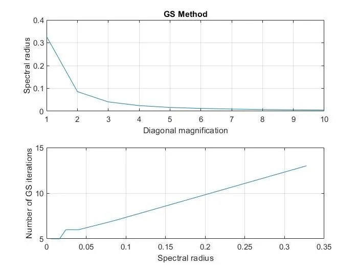
• Gauss-Seidel Method

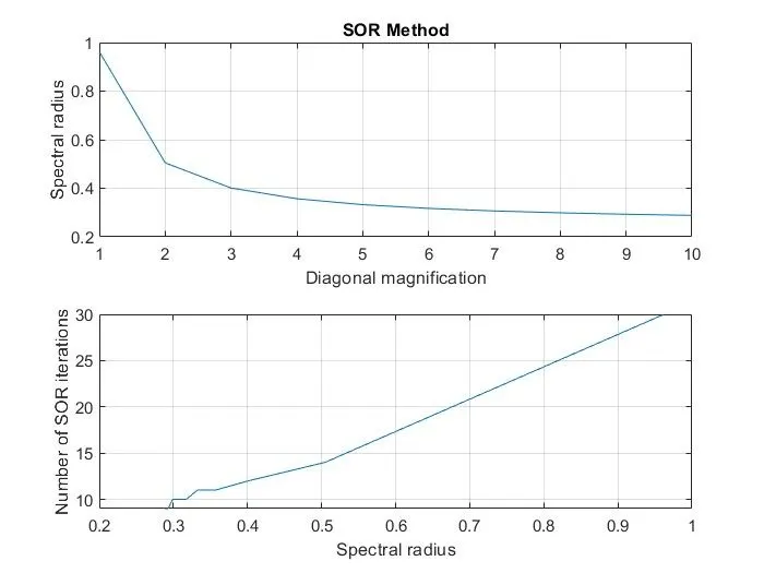
• SOR Method

CONCLUSIONS

• When the diagonal magnification increases, the value of the spectral radius decreases.
• Also when the spectral radius increases, the number of iterations also increases.
• When the spectral radius in any method is greater than 1, then the number of iterations for convergence decreases and we get an unstable solution. We can observe that for small values of magnification factor. Plots for that inference are attached with the report separately