Tire Modeling - Pacjecka Magic Tire Formula and Combined Slip brush tire model

Problem Set 2a

Write an Octave script to show the effect of slip angles (2 through 10 deg in increments of 2) on the Fx vs Fy relationship.
Use a slip ratio range of 0 to 1 (or 0 to 100%)
Use the combined slip brush tire model we developed in class. Develop your script based on the algorithm. These are your deliverables:
1. Plot showing the effect of different slip angles on Fx vs Fy relationship
2. Inference from the plot

Theory of Combined-slip model: The longitudinal and lateral tire brush models explained these forces individually. But in reality, these forces occur simultaneously during vehicle manueuvers like braking in aturn. Therefore the tire model must be able to deal with combined tractive and cornering forces, such a situation is called as comprehensive slip. The model gives us the relationship between the longitudinal force and lateral forces at various slip angles and slip ratios. It is depicted by a diagram called as the friction circle. The resultant force, otherwise known as the maximum road plane force is equal to the radius of the curve, which is equal to the product of coefficient of friction (mu) and the vertical load (Fz) acting on the tires.

Octave code:

The coding logic is as follows :

- Input all the given data and then calculate the longitudinal and cornering stiffness.

- Create a for-loop inorder to calculate the forces for various slip angles from 2 to 10 degrees, in increments of 2 degrees.

- For varying skid/slip ratio from 0 to 1 , the critical length is calculated and based on whether it is smaller or larger than the contact patch length, the appropriate formulas lateral and longitudinal forces are used.

- Finally plot the values of lateral and longitudinal forces for different slip angles.

% combined braking and cornering 

clear all 

Fz =4000 ; % Normal force (N)
mu =0.85 ; % Peak road-tire friction coefficient
lt =0.2 ; % length of tire contact patch (m)
kt =3.5e6 ; % tire tangential stiffness (N/m^2)
ky = 2.5e6 ; % tire cornering stiffness (N/m^2)

%Compute Cx,Cy
C_x= (lt^2*kt)/2;
C_alpha = (lt^2*ky)/2;

for i=2:2:10 % slip angle from 2 to 10 in increments of 2 degrees.
 alpha = i*(pi/180);
 
 for j=1:201
  Sb =(j-1)*0.005; %skid ratio array from 0 to 1 
  temp = (((C_x*Sb)^2) + ((C_alpha*tan(alpha))^2))^0.5; 
  lc = ((mu*Fz)*(1-Sb)*lt)/(2*temp); % critical length 
  
  if lc >=lt
    Fx(j) = (c_x*Sb)/(1-Sb);
    Fy(j) = (C_alpha*tan(alpha))/(1-Sb);
  else
    Fx(j) = ((mu*Fz*C_x*Sb)/temp)*(1-((mu*Fz*(1-Sb))/(4*temp)));
    Fy(j) = ((mu*Fz*C_alpha*tan(alpha))/temp)*(1-((mu*Fz*(1-Sb))/(4*temp)));
  end
 
end 

plot(Fx,Fy,'linewidth',3);
hold on;
 
end

set(gca,'fontsize',15);
title('Combined slip - lateral force vs longitudinal force');
xlabel('longitudinal force Fx(N)');
ylabel ('Lateral force Fy(N)');
legend ('2deg','4deg','6deg','8deg','10deg');

Plot showing the effect of different slip angles on Fx vs Fy relationship.

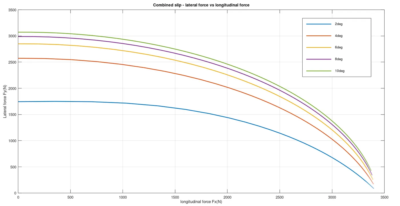
Inference: The plot gives us the g-g diagram or the friction circle which illustrates the longitudinal force Fx and lateral force Fy as a function of variosu slip angles. It is the performance envelope of the vehicle. The X-axis represents the longitudinal force and the Y-axis depicts the lateral force, the curves represent the maximum operating points at various slip angles. As long as the vehicle operating point is within the ellipse, there wont be any skidding or sliping, if the point moves out then the vehicle starts to skid or slip. The resultant peak force generated at the tires, is governed by the radius of the curve. The curves are elliptical in shape as the tire's lateral and longitudinal force generating capabilities are not the same. The general equation of the ellipse is :

`(F_x/(F_(xmax)))^2+(F_y/(F_(ymax)))^2=1` Where Fx and Fy are the longitudinal and lateral forces. Fxmax and Fymax are the maximum longitudinal and lateral forces generated by the tire at a particular slip angle.

As the slip angle increases , the maximum lateral force generated by the tire keeps increases, whereas the maximum longitudinal force remains more or less the same at various slip angles. At a particular slip angle, the lateral force increases as the longitudinal decreases or vice-versa. Say for example in a cornering situation, in the mid corner when we start to accelerate our way out of the turn, both traction and cornering forces are present, in such cases as we accelerate the vehicle, as the traction force keeps increasing, there is a loss of lateral force. This loss of lateral force casues the radius of the turn to increase, thereby affecting the steering of the vehicle.

Problem Set 2b – combined slip – abs and side force

This challenge tests your understanding of combined slip brush tire model
This exercise should be done in octave. Turn in your code
Write an Octave script to calculate the effective cornering stiffness under different slip ratios (0, 0.15 and 1.0) and fixed slip angle (3 deg)
Use the combined slip brush tire model we developed in class. Develop your script based on the algorithm we looked at in class. These are your
deliverables:
1. Effective cornering stiffness values
2. Inference from the plot

Problem Set 2b – combined slip – abs and side force

In this case plot the cornering stiffness vs the slip ratio has to be generated at a particular slip angle (3 degrees).

Cornering stiffness is the slope of the lateral force vs slip angle graph. In otherwords, its the ratio between the lateral force and slip angle. The slip angle is 3 degrees in this case. The lateral force is calculated using the formulas derived in the combined slip brush tire model. The formula varies depending on whether its the adhesion region or the slipping (large excitation) region.

The octave code to calculate this is as follows, the cornering stiffness is calculated and is plotted against the slip ratio. The coding logic is described inside the scipt ,before each step in the program.

% combined braking and cornering 

clear all 

Fz =3000 ; % Normal force (N)
mu =0.8 ; % Peak road-tire friction coefficient
lt =0.2 ; % length of tire contact patch (m)
kt =4.0e6 ; % tire tangential stiffness (N/m^2)
ky = 2.275e6 ; % tire lateral stiffness (N/m^2)

%Compute longitudinal stiffness (C_x) and lateral stiffness (C_y)
C_x= (lt^2*kt)/2;
C_alpha = (lt^2*ky)/2;

for i=3 % slip angle is fixed at 3 degrees.
 alpha = i*(pi/180);
 
 
 for j=1:201
  Sb(j) =(j-1)*0.005; %skid ratio array from 0 to 1
  temp = (((C_x*Sb(j))^2) + ((C_alpha*tan(alpha))^2))^0.5; 
  lc = ((mu*Fz)*(1-Sb(j))*lt)/(2*temp); % critical length is calculated 
  
  % critical length is compared with the contact patch length, as the formula of lateral force varies based on whether its a adhesion region or slipping (large excitation) region.

  if lc >=lt
     Fy(j) = (C_alpha*tan(alpha))/(1-Sb(j));
  else
     Fy(j) = ((mu*Fz*C_alpha*tan(alpha))/temp)*(1-((mu*Fz*(1-Sb(j)))/(4*temp)));
end
C_y=Fy/i; % cornering stiffness is the ratio between lateral force and slip angle (N/deg);

end 
end

% the cornering stiffness vs slip ratio graph is plotted. This indicates the value of cornering stiffness at various slip ratios.
plot(Sb,C_y,'linewidth',3);
set(gca,'fontsize',15);
title('Cornering stiffness vs Slip ratio');
xlabel('Slip ratio');
ylabel ('Cornering stiffness(N/deg)');
grid on;
hold on;

% cornering stiffness values at slip ratios of 0,0.15,1
C_y1=Fy(1)/3 %Fy(1) is the lateral force at slip ratio=0
C_y2=Fy(31)/3 %Fy(31) is the lateral force at slip ratio=0.15
C_y3=Fy(201)/3 %Fy(201) is the lateral force at slip ratio=1.00
C_yt = [C_y1,C_y2,C_y3];
slip_ratio = [0,0.15,1];

%plotting the points specified. 
plot(slip_ratio,C_yt,'o','MarkerFaceColor','r','MarkerSize',8);
hold off;

Graph between the effective cornering stiffness values vs slip ratio.

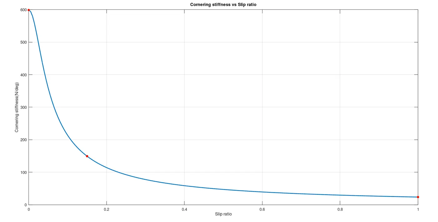
The values of effective cornering stiffness at various slip ratios is as follows :

- at slip ratio 0 = 598.70 N/deg.

- at slip ratio 0.15 = 149.42 N/deg.

- at slip ratio 1 = 23.835 N/deg.

Inference: As the slip increases the cornering stiffness value reduces. Therefore, the lateral force also decreases. As it can be seen in this example, there is a loss of 75% of lateral force as the slip increases from 0 to 0.15.The decreasing trend of lateral force indicates the slips have to be limited to guarantee the lateral guidance of the vehicle. When lateral and longitudinal forces act simultaneously, increasing the slip angle to achieve the maximum longitudinal force, will result in reducing the lateral force to an unacceptable level, because if lateral force decreases beyond a limit, the vehicle stability is lost.

The ABS system aims at minimizing the braking distance while retaining steering ability during braking. For optimum performance of the braking system usually ABS control system are operated at a working range wherein a desired slip is determined when the braking force is maximum and there is enough lateral force to maintain vehicle stability and the control system is programmed to maintain the slip at that desired level.

Problem Set 2c – pacjecka Mz

This challenge tests your understanding of curve fitting using the Pacjecka magic formula. This exercise should be done in octave.
The file “tire_test_data” contains slip angle and aligning torque data.

Using the magic tire formulation, obtain fit coefficients so that your curve describes the tire test data accurately. Write a post-processing routine to calculate the RMS error of the curve fit. Tune your coefficients so that the RMS error is less than 2.0 Nm. Deliverables are as follows :
1. Coefficients that meet the RMS criteria
2. Plot showing the curve fit
3. RMS calculation

Problem Set 2c – pacjecka Mz

Magic Tire Formula : This model empirically represents and interpolates previously measured tire forces and moment curves. In this model, the curves are obtained beforehand experimentally, then curve fitting is done to obtaine the formula of the curve. This curve equation is then further used in simulation works. A common formula is developed using mathematical function which relates :

- Lateral force and slip angle.

- Longitudinal force and slip ratio.

- Aligning moment and slip angle.

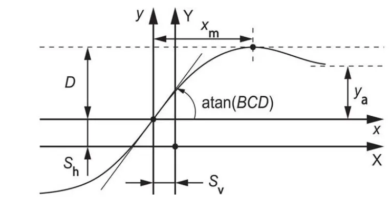
`Y(x)=D⋅sin[C⋅arctan(Bx−E(Bx−arctan(Bx)))]` where `Y(x)=y(x)+S_vandx=X+S_h` .

'y' is the forces and moments while 'x' is the slip angle and slip ratio. 'B" is the stiffness factor, 'C' is shape factor, 'D' represents the peak value, 'E' is the curvature factor, 'S_h and S_v' are the offset from the origin inorder to account for the camber thrust, plysteer and conicity. 'BCD' represents the slope of the curve. Each of these factors are related to the vertical load acting on the tire.

Octave Code : The coding logic is described inside the scipt ,before each step in the program.

% Magic formula - curve fitting for aligning moment vs slip angles.
clear all ;

%the tire test data is loaded into the script
load tire_test_data;

%The aligning moment and slip angle values are seperated.
a = tire_test_data(:,1);   % slip angle (degrees)
Mz = tire_test_data(:,2);   % aligning moment (Nm)

%plot the test data 
plot(a,Mz);
title('Aligning moment vs slip angle','fontsize',18);
xlabel('Slip angle (deg)','fontsize',18);
ylabel('Aligning moment (Nm)','fontsize',18);
set(gca,'fontsize',15);
hold on

% pac coefficients are first calculated using formulas and other relations, and then with that as the starting point are further tuned to obtain a minimum value of RMS error.

D = 59.64; 
%Xm = 3.3 deg. Xm the slip angle at which peak alignign moment is achieved.
C = 2.165 ; %(aligning moment)
slope = 26.93;
B = (slope/(C*D)) ;;
%E = -2.3246 ; 
Shy = 0 ;
Svy = -0.4 ;
E = ((B*3.3)-(tan(pi/(2*C))))/((B*3.3)-(atan(B*3.3)));

%The slip angles from the tire data are taken and substituted into the magic tire formula and according to the formula an aligning moment data set is obtained based on the pac-formula/ magic tire formula.

for i=1:278
  %A1(i) = a1(i) + Shy; %to include the horizontal shift
  A1(i)=a(i);
  Mz1(i) = D*sin(C*atan(B*A1(i)-E*(B*A1(i)-atan(B*A1(i)))));
  MZ1(i) = Mz1(i) + Svy;
  
%Mz is the aligning moment from tire test data, while MZ1 is the aligning moment from the magic formula. The difference in both is the error in the fit.

  error_sq(i) = (Mz(i) - MZ1(i))^2;
  
end

%plot the magic formula data 
plot(A1,MZ1);
legend('Test data','Pac formula');
grid on;
hold off;

%rms value calculation- To calculate it first the error term is squared, then to obtainf the mean its divided by the total number of data points. Then the square root is taken to get the RMS error value. 

rms_value = sqrt(sum(error_sq)/i);

The value of D is the peak value of the test data curve. Since there is a loading and unloading curve, the peak value is taken as the average of both these curves, hence the starting point for D is kept at 59.28. The value of C is kept as 2.4 (default value for aligning moment). The slope of the curve is calculated.

The value of B is equal to [slope / (C*D)]. The value of E is given by a formula : [B*xm -tan(pi/2C)]/[B*xm - atan(B*xm)]. Where xm is the slip angle at which peak aligning moments is achieved. These values serve as the starting points, further they are tuned to achieve a better fit, with a lower RMS error value.

The coefficient values after tuning are :

B = 0.20856

C = 2.165 (with the default value of 2.4 the RMS error was higher(2.8451Nm) than the target(2Nm)).

D= 59.64

E= -2.3246

S_h =0

S_v = -0.4

RMS error value : The given data has values of aligning moment for various slip angles. Through the magic tire formula, a data set is obtained. For the same slip angles, the two values of aligning moments (tire data set and the other from pac-formula) are compared.

Root mean square value = `sqrt((M_Z - M_(z1))^2/n)`

Where 'Mz' is the alignign moment value from the tire data, 'MZ1' is the aligning moment value obtined from the magic tire formula, and 'n' is the total number of data points being compared. The value of this error is 1.8643 Nm.

Output Graph:

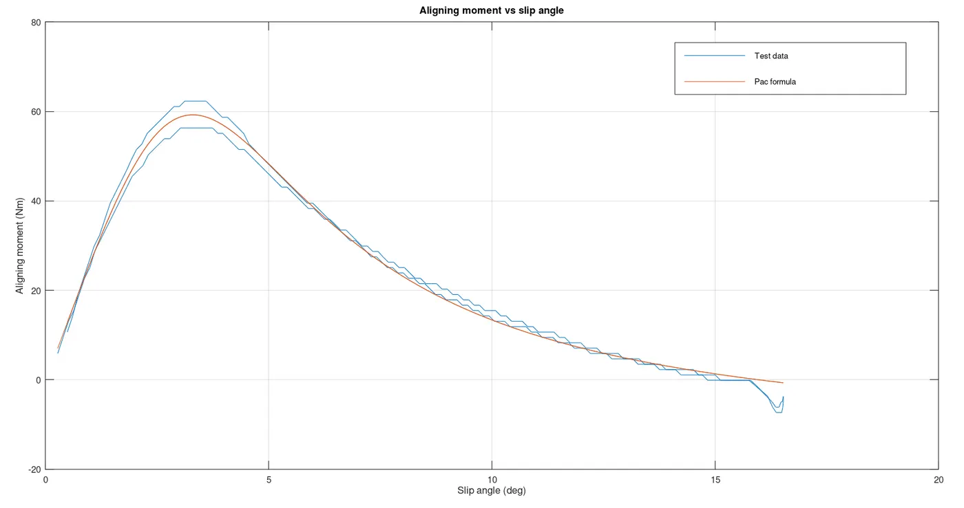
Inference: The graph is the plot between aligning moment and slip angle. The magic tire formula is used, the coefficient are tuned to obtain a good fit of the tire data. This curve fitted can be further used for simulation works.