Supervised Learning - Prediction Week 3 Challenge

• Perform Gradient Descent in Python with any loss function

Gradient Descent is an optimization algorithm in machine learning used to minimize a function by iteratively moving towards the minimum value of the function.We basically use this algorithm when we have to find the least possible values that can satisfy a given cost function. In machine learning, more often that not we try to minimize loss functions. By minimizing the loss function , we can improve our model, and Gradient Descent is one of the most popular algorithms used for this purpose.

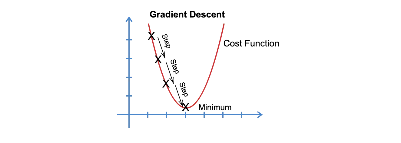
We first take a point in the cost function and start moving in steps towards the minimum point. The size of that step, or how quickly we have to converge to the minimum point is defined by Learning Rate. We can cover more area with higher learning rate but at the risk of overshooting the minima. On the other hand, small steps/smaller learning rates will consume a lot of time to reach the lowest point.

PYTHON CODE-

#import the basic modules
import numpy as np
import matplotlib.pyplot as plt
from scipy.constants.codata import precision

#creating the function and plotting it We will find the gradient decent of this function - f(x) = x^3-3x^2+7
function = lambda x: (x ** 3)-(3 *(x ** 2))+7

#Get 1000 evenly spaced numbers between -1 and 3 (arbitratil chosen to ensure steep curve)
x = np.linspace(-1,3,500)

#Plot the curve
plt.plot(x, function(x))
plt.show()

#This function takes in a value of x and returns its derivative based on the initial function specified.
def deriv(x):
    x_deriv = 3* (x**2) - (6 * (x))
    return x_deriv

#This function takes in an initial or previous value for x, updates it based on steps taken via the learning rate and outputs the most minimum value of x that reaches the precision satisfaction.
def step(x_new, x_prev, precision, l_r):
    
    # create empty lists where the updated values of x and y wil be appended during each iteration
    x_list, y_list = [x_new], [function(x_new)]
    
    # keep looping until your desired precision
    while abs(x_new - x_prev) > precision:
        
        # change the value of x
        x_prev = x_new        
        # get the derivation of the old value of x
        d_x = - deriv(x_prev)        
        # get your new value of x by adding the previous, the multiplication of the derivative and the learning rate
        x_new = x_prev + (l_r * d_x)        
        # append the new value of x to a list of all x-s for later visualization of path
        x_list.append(x_new)
        # append the new value of y to a list of all y-s for later visualization of path
        y_list.append(function(x_new))
        
    print ("Local minimum occurs at: "+ str(x_new))
    print ("Number of steps: " + str(len(x_list)))
    
    plt.subplot(1,2,2)
    plt.scatter(x_list,y_list,c="g")
    plt.plot(x_list,y_list,c="g")
    plt.plot(x,function(x), c="r")
    plt.title("Gradient descent")
    plt.show()

    plt.subplot(1,2,1)
    plt.scatter(x_list,y_list,c="g")
    plt.plot(x_list,y_list,c="g")
    plt.plot(x,function(x), c="r")
    plt.xlim([1.0,2.1])
    plt.title("Zoomed in Gradient descent to Key Area")
    plt.show()

#Implement gradient descent (all the arguments are arbitrarily chosen)    
step(0.5, 0, 0.001, 0.05)    
        

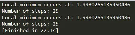
Local minimum occurs at: 1.9980265135950486
Number of steps: 25

• Difference between L1 & L2 Gradient descent method

• What are the different loss functions for regression
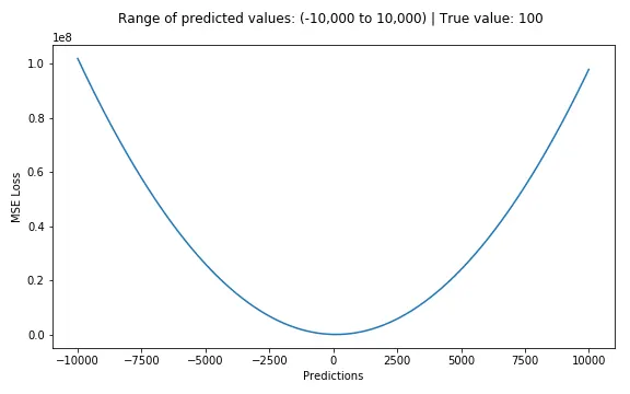
• Mean Square Error- It is the most commonly used regression loss function. As the name suggests, Mean square error is measured as the average of squared difference between predictions and actual observations. It’s only concerned with the average magnitude of error irrespective of their direction. However, due to squaring, predictions which are far away from actual values are penalized heavily in comparison to less deviated predictions.

Below is a plot of an MSE function where the true target value is 100, and the predicted values range between -10,000 to 10,000.

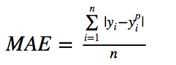
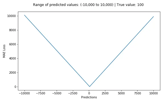
• Mean Absolute Error, L1 Loss- MAE is the sum of absolute differences between our target and predicted variables. So it measures the average magnitude of errors in a set of predictions, without considering their directions. The range is also 0 to ∞.

• Huber or Smooth Mean Absolute Error-Is less sensitive to outliers in data than the squared error loss. It’s also differentiable at 0. It’s basically absolute error, which becomes quadratic when error is small. How small that error has to be to make it quadratic depends on a hyper-parameter, 𝛿 (delta), which can be tuned. Huber loss approaches MAE when 𝛿 ~ 0 and MSE when 𝛿 ~ ∞ .

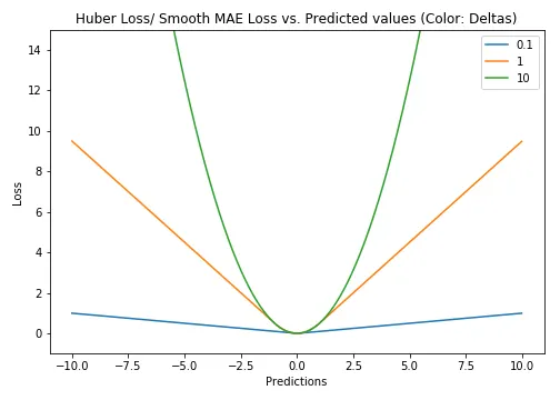
One big problem with using MAE for training of neural nets is its constantly large gradient, which can lead to missing minimal at the end of training using gradient descent. For MSE, gradient decreases as the loss gets close to its minimal, making it more precise.Huber loss can be really helpful in such cases, as it curves around the minimal which decreases the gradient. And it’s more robust to outliers than MSE. Therefore, it combines good properties from both MSE and MAE.

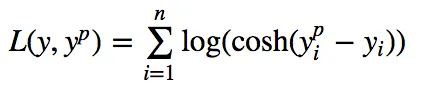
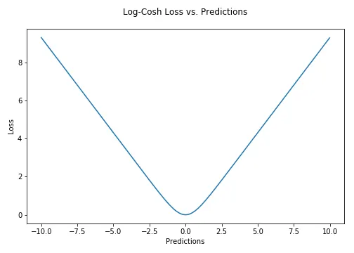
• Log-Cosh Loss- Log-cosh is the logarithm of the hyperbolic cosine of the prediction error.Its smoother than L2.

• What is the importance of learning rate

Learning rate is a scalar, a value which tells the machine how fast or how slow to arrive at some conclusion. The speed at which a model learns is important and it varies with different applications. A super fast learning algorithm can miss a few data points or correlations which can give better insights on the data.It is a tuning parameter in an optimization algorithm that determines the step size at each iteration while moving toward a minimum of a loss function.

-A smaller learning rate may allow the model to learn a more optimal or even globally optimal set of weights but may take significantly longer to train.

-Learning rate gives the rate of speed where the gradient moves during gradient descent. Setting it too high would make your path instable, too low would make convergence slow.

• How to evaluate linear regression

There are a number of metrics used in evaluating the performance of a linear regression model. They include:

• R-Squared: seldom used for evaluating model fit, itis also known as the coefficient of determination, itmeasures the percentage of variation in the response (dependent) variable explained by the predictor in the predictor (independent) variable. it has values between 0 and 1 for every single regression. Where values between 0.3 and 0.5 refer to a weak r-squared, 0.5 and 0.7 refers to a moderate r-squared, and values > 0.7 refer to a strong r-squared. the higher the r-squared, the better the model fits your data (there is a caveat to this…) because there is a possibility of having a low r-squared value for a good model and vice-versa.it is a relative measure of model fit. This means they are not a good measure to determine how well a model fits the data.

sklearn module : sklearn.metrics.r2_score

mathematical formula: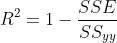

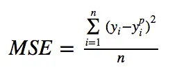
• MSE (Mean Squared Error): used for evaluating model fit, it measures the average of the squared difference between the observed value and the actual value. a value of 0 indicates a perfect fit, this means that the data predict the outcome accurately, however in most cases, it is hardly ever so.

sklearn module: sklearn.metrics.mean_squared_error

mathematical formula:

• RMSE (Root Mean Squared Error): always used for evaluating model fit.is the measure of the distance between the actual values and the predicted value. the lower the RMSE the better the measure of fit. This means that there is little variation in the spread of data. it is a good measure of how accurately the model predicts the target, it is considered the best statistics to determine the relationship between the model and the response variable, it measures the spread of the data points from the regression line.

using sklearn and math module to perform RMSE

from sklearn.metrics import mean_squared_error

from math import sqrt

rmse = sqrt(mean_squared_error(y_actual, y_predicted))

print(rmse)

mathematical formula

• What is the difference between multiple and adjusted coefficient of determination

R² measures the proportion of the total variation in Y explained by the regression model.

Here are some key points about R²:

• It is a non-negative quantity with range 0 ≤ R² ≤ 1
• R² = 0 implies that the regression line does not fit the data at all.
• R² = 1 implies that the regression line is a perfect fit.

Adjusted R² is a modified version of R² adjusted with the number of predictors. It penalizes for adding unnecessary features and allows a comparison of regression models with a different number of predictors. The adjusted R-squared increases only if the new term improves the model more than would be expected by chance. It decreases when a predictor improves the model by less than expected by chance.

Obtaining a negative value for Adjusted R² can indicate few or all of the following:

• The linear model is a poor fit for the data
• The number of predictors is large
• The number of samples is small