Classification Surface defects in stainless steel plates using SVM algorithm

1) Pros and cons of SVM

Pros :

• Works well for high dimensional problems
• Since it calculates using support vectors the computational memory is low

Cons :

• Does not work well for a large amount of data
• Does not work well if the target classes are overlapped

2) Apply SVM to the “Surface defects in stainless steel plates” dataset and evaluate it

Aim :

To apply SVM algorithm on the surface defects in stainless steel plates dataset and evaluate it

Methods :

Descriptive analysis :

The given dataset is imported into python. The dataset is printed to get an idea

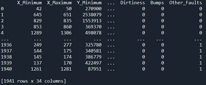
So there are 1941 rows and 34 columns, Now we print all column names

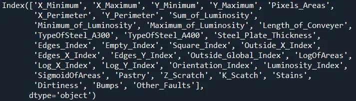
So there are 27 features and the faults are represented in the last 7 columns using one hot encoding

Now lets try to get info on the dataset

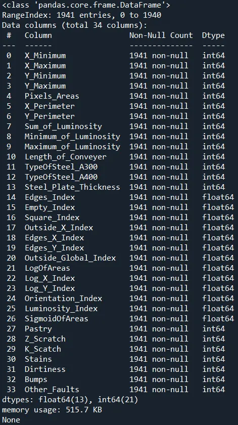
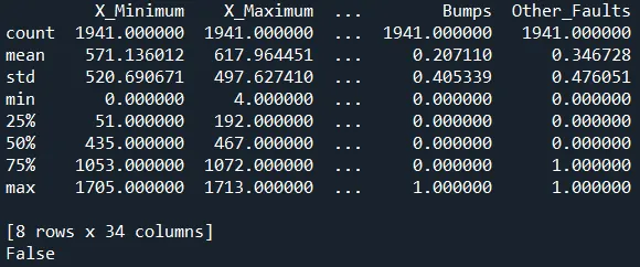
We check for null values and found there are no null values

Since there are many features we can remove some features which almost similar to other features, we can find this by plotting a correlation matrix

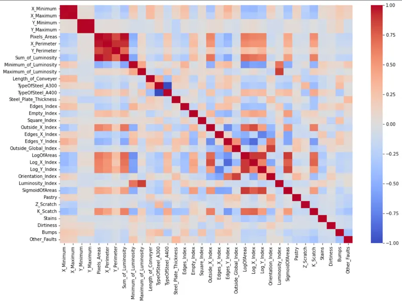
So the areas which are close to the value 1 are closely related and hence can be removed to avoid repetition in the features

From the above figure we can say that

• x_minimum is related to x_maximum
• y_minimum is related to y_maximum
• pixel_areas is related to x_perimeter and sum_of_luminosity
• Logofareas is related to Log_X_index, Log_y_index and Sigmoidof areas
• Luminosity index is related to maximum_of_luminosity
• Orientaion index and outside_global_index

So if we drop the related columns we end up with

Now lets plot histogram of each feature to see the variation in the features

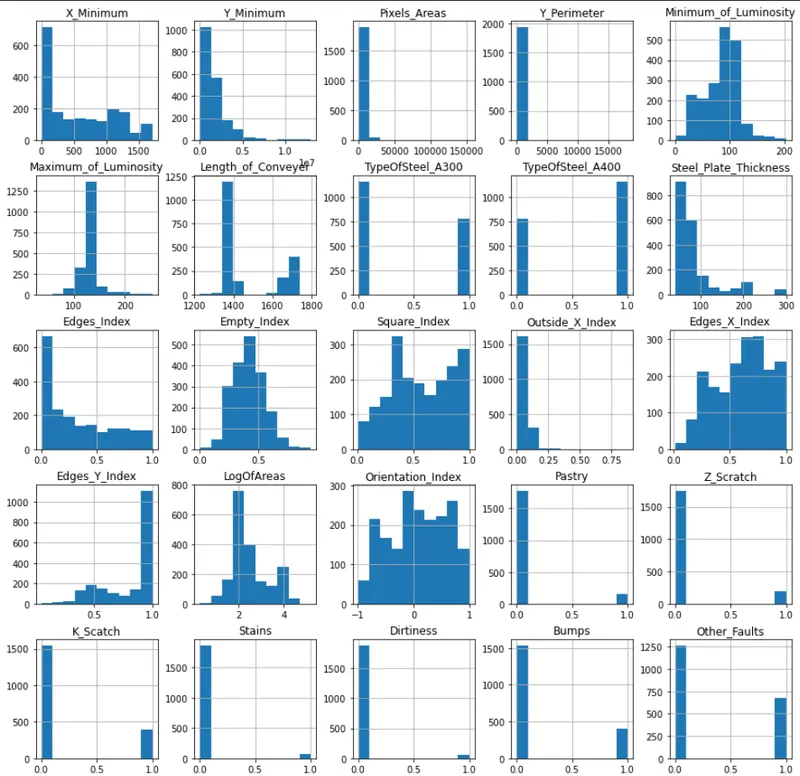
To find outliers we can use boxplot

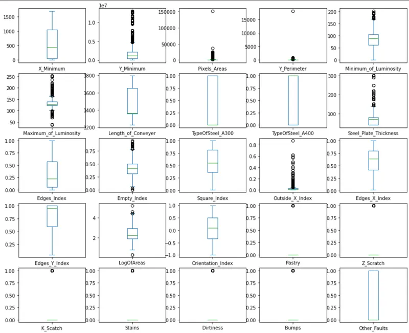
We don't change the values for the outliers because we need experimental data to get correct results

Diagnostic analysis :

So now we look at the faults and number of faults in each classes using bar graph

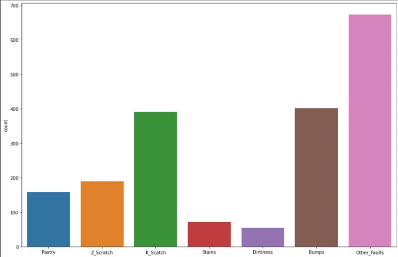
We can see the counts of each fault with other_faults having the maximum count

Predictive analysis :

Code :

import pandas as pd
import matplotlib.pyplot as plt
import seaborn as sns
df=pd.read_csv("faults.csv")
print(df)
print(df.columns)
print(df.info())
print(df.describe(include="all"))
print(df.isnull().values.any())
plt.figure(figsize=(15,10))
sns.heatmap(df.corr(),cmap="coolwarm")
df=df.drop(['X_Maximum','Y_Maximum','X_Perimeter','Log_X_Index','Sum_of_Luminosity','Log_Y_Index','SigmoidOfAreas','Luminosity_Index','Outside_Global_Index'],axis=1)
print(df.shape)
df.hist(figsize=(15,15))
df.plot(kind='box',layout=(6,5),subplots=True,sharex=False,sharey=False,figsize=(15,15))
columns_label=df.columns.values[-7:]
print(columns_label)
targets=(df.iloc[:,-7:]==1).idxmax(1)
print(targets)
sns.countplot(targets)
x=df.iloc[:,0:18]
print(x)
from sklearn.preprocessing import StandardScaler
sc=StandardScaler()
X=sc.fit_transform(x)
from sklearn.model_selection import train_test_split
x_train,x_test,y_train,y_test=train_test_split(X,targets,test_size=0.1,random_state=9)
from sklearn import svm
r=svm.SVC(C=1,kernel='linear',gamma='auto')
r.fit(x_train,y_train)
print(r.score(x_test,y_test))
y_p=r.predict(x_test)
from sklearn import metrics
cm=metrics.confusion_matrix(y_test, y_p)
print(cm)
sns.heatmap(cm,annot=True)
plt.xlabel("Predicted")
plt.ylabel("Actual")
plt.show()

So the following accuracy was found for different training and test spilt

Training-Test Split	Training Accuracy	Test Accuracy
90-10%	73.9%	73.8%
80-20%	73.8%	72.7%
70-30%	74.9%	73.4%

So we can see the underfitting issue here

Prescriptive analysis :

The confusion matrix was visualized

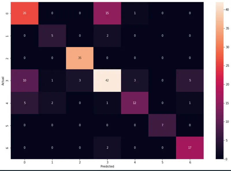
So the majority of misclassification was done as stains, hence there may be some wrong data in stains. To improve accuracy one can also try running the simulation with the more features