STUDY OF LONGITUDINAL & LATERAL FORCES WITH THE PACJECKA MAGIC TIRE MODEL IN MATLAB

This project aims at studying how different slip angles influence the forces (Fx and Fy) vs slip ratio (sweep from 0 to 60%) and how different slip ratios influence the force (Fx and Fy) vs slip angle (sweep from 0 to 20 deg) using the Modified slip approach in Pacjecka Magic tire model in MATLAB.

Aim:

1. To study how different slip angles (0 deg, 2 deg, 4 deg and 6 deg) influence the force (Fx and Fy) vs slip ratio relationship (sweep from 0 to 60%).

2. To study how different slip ratios (0%, 3%, 6% and 9%) influence the force (Fx and Fy) vs slip angle relationship (sweep from 0 to 20 deg).

Objectives:

Using the modified slip approach,

1. Plot showing the effect of different slip ratios on lateral force vs slip angle relationship

2. Plot showing the effect of different slip ratios on longitudinal force vs slip angle relationship

3. Plot showing the effect of different slip angles on longitudinal force vs slip ratio relationship

4. Plot showing the effect of different slip angles on lateral force vs slip ratio relationship

INPUTS:

Download the .mat file containing this data here: Pacjecka_model_parameters

Just remember to put this in the same folder as the below Matlab code.

You can change the values of the parameters within the Matlab workspace window.

Matlab Code: Main

close all
clear all
clc

load('pacjecka_model_parameters')

% Pacjecka Magic Modeling for variable slip ratios
Fx = zeros();zeros(); Fy = zeros();zeros(); a = zeros();
for i = 1:4
    s = (i-1)*0.03; % Slip ratios 0, 3, 6, 9
    for j = 1:201
        a(j) = (j-1)*0.1; % Slip angles
        
        sol = pacjecka_magic_formula(ps,pa,By,Cy,Dy,Ey,Shy,Svy,Bx,Cx,Dx,Ex,Shx,Svx,s,a(j)); % Pacejka magic formula
        Fx(i,j) = sol(:,1); % Lateral force
        Fy(i,j) = sol(:,2); % Longitudinal force
    end
end

% Plotting
figure(1)
subplot(2,1,1)
plot(a,Fy,'Linewidth',1.5)
title('Lateral force V/S Slip angle')
xlabel('Slip angle (degrees)')
ylabel('Lateral force (N)')
legend('0% Slip','3% Slip','6% Slip','9% Slip','Location','Southeast')
grid on
subplot(2,1,2)
plot(a,Fx,'Linewidth',1.5)
title('Longitudinal force V/S Slip angle')
xlabel('Slip angle (degrees)')
ylabel('Longitudinal force (N)')
legend('0% Slip','3% Slip','6% Slip','9% Slip')
sgtitle('VARIABLE SLIP RATIOS')
grid on
saveas(1,'Slip ratio Fx Fy','png')

clear all

load('pacjecka_model_parameters')

% Pacjecka Magic Modeling for variable slip angles
Fx = zeros();zeros(); Fy = zeros();zeros(); a = zeros();
for i = 1:4
    a = (i-1)*2; % Slip angles 0, 2, 4, 6 degrees
    for j = 1:300
        s(j) = (j-1)*0.002; % Slip ratios
        
        sol = pacjecka_magic_formula(ps,pa,By,Cy,Dy,Ey,Shy,Svy,Bx,Cx,Dx,Ex,Shx,Svx,s(j),a); % Pacejka magic formula
        Fx(i,j) = sol(:,1); % Lateral force
        Fy(i,j) = sol(:,2); % Longitudinal force
    end
end

% Plotting
figure(2)
subplot(2,1,1)
plot(s,Fy,'Linewidth',1.5)
title('Lateral force V/S Slip ratio')
xlabel('Slip ratio')
ylabel('Lateral force (N)')
legend('0 deg','2 deg','4 deg','6 deg')
grid on
subplot(2,1,2)
plot(s,Fx,'Linewidth',1.5)
title('Longitudinal force V/S Slip ratio')
xlabel('Slip ratio')
ylabel('Longitudinal force (N)')
legend('0 deg','2 deg','4 deg','6 deg','Location','Southeast')
sgtitle('VARIABLE SLIP ANGLES')
grid on
saveas(2,'Slip angle Fx Fy','png')

Matlab Code: Pacjecka function

function [sol] = pacjecka_magic_formula(ps,pa,By,Cy,Dy,Ey,Shy,Svy,Bx,Cx,Dx,Ex,Shx,Svx,s,a)
    % Normalized slip factors
    s_norm = s/ps;
    a_norm = a/pa;

    % Resultant slip
    s_res = sqrt(s_norm^2 + a_norm^2);

    % Modified slip factors
    s_mod = s_res*ps;
    a_mod = s_res*pa;

    % Lateral force
    A = a_mod + Shy;
    FY = a_norm/s_res;
    Fy = Dy*sin(Cy*atan(By*A-Ey*(By*A-atan(By*A))))*FY + Svy;

    % Longitudinal force
    Ax = s_mod + Shx;
    FX = s_norm/s_res;
    Fx = Dx*sin(Cx*atan(Bx*Ax-Ex*(Bx*Ax-atan(Bx*Ax))))*FX + Svx;
    
    sol = [Fx,Fy];
end

Code Logic:

1. Create a .mat file containing the model parameters using the save() function in Matlab.
2. Load this file, the code now reads the input values. These can be edited in the workspace window.
3. For variable slip ratios, create a primary loop of up to 4 iterations. Each iteration value is subtracted by 1 and multiplied by 0.03 to get 0, 0.3, 0.6 and 0.9 slip ratios.
4. For variable slip angles, create a primary loop of up to 4 iterations. Each iteration value is subtracted by 1 and multiplied by 2 to get 0, 2, 4 and 6 degrees of slip angle.
5. The forces are calculated using Pacjecka's magic formula.

Plots:

1.

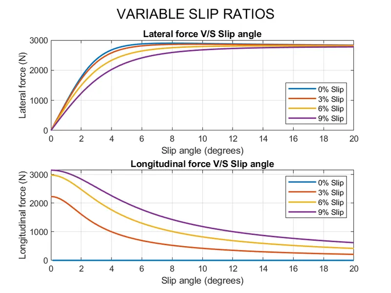
Inference from the plot: (Different slip ratios)

(i) Lateral force v/s Slip angle

- The lateral force increases with an increase in the slip ratio until the peak slip angle post which the curve saturates.

- There is 0 N lateral force at a 0-degree slip angle at all levels of slip ratio.

- There is a maximum variation in the lateral forces at a slip angle +/-2 of the peak slip angle.

ii) Longitudinal force v/s Slip angle

- The longitudinal force is 0 N at a 0% slip ratio for all slip angles.

- The longitudinal force kind of decreases with an increase in slip angle.

- The Maximum longitudinal force is achieved at 0 slip angle. And it decreases with an increase in slip angle.

- The greater the slip ratio, the higher the longitudinal force until it reaches the max slip ratio. Post which it will saturate.

2.

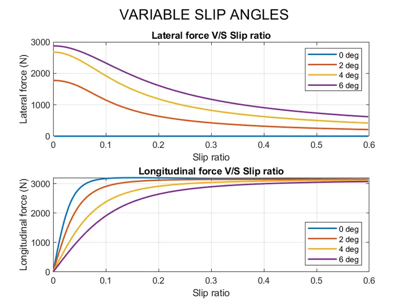
Inference from the plot: (Different slip angles)

(i) Lateral force v/s Slip ratio

- The lateral force is 0 N at a 0% slip angle for all the slip ratios.

- The lateral force kind of decreases with an increase in slip ratio.

- The Maximum lateral force is achieved at a 0 slip ratio. And it decreases with an increase in slip ratio.

- The greater the slip angle, the higher the longitudinal force until it reaches the max slip angle. Post which it will saturate.

- The Lateral force V/S Slip ratio plot with variable slip angle is similar to the Longitudinal force V/S Slip angle with variable slip ratio.

(ii) Longitudinal force v/s Slip ratio

- The longitudinal force increases with an increase in the slip ratio until the peak slip ratio, post which the curve saturates.

- There is 0 N longitudinal force at a 0-degree slip ratio at all slip angles.

- There is a maximum variation in the lateral forces at a slip ratio +/-0.5 of the peak slip ratio.

- The longitudinal force V/S Slip ratio plot with variable slip angle is similar to the Lateral force V/S Slip angle with variable slip ratio.

References:

1. Pacjecka magic tire model using MATLAB by Roshan