Curve fitting

Curve fitting is the method of capturing the trend in the data and creating a curve by assigning a single function across the entire range to identify the coefficients ‘a’ and ‘b’ such that f(x) ‘fits’ the data well.

I. AIM

To write code to fit a linear and cubic polynomial for the Cp data.

II. OBJECTIVES

1. Write a code to predict the specific heat curve with respect to the temperature.
2. To write a code that uses the splits method to predict the specific heat curve.
3. Calculate the fitness of the curve fit.

IV. MATLAB CODE

IV.1. MATLAB CODE WITH NORMALIZING

data = load('data'); % Copy the data of data file into data array

% Segrigating the data
temp_data = data(:,1); % Temperature values
cp_data = data(:,2); % Specific heat values

% Scaling and centering the x-axis variables which is the temperature here
temp_scale = normalize(temp_data,'scale'); % Scaling
temp = normalize(temp_scale,'center','mean'); % Centering

co_effs_linear = polyfit(temp_scale,cp_data,1); % Coefficeint values to generate a linear curve
predicted_cp_linear = polyval(co_effs_linear, temp_scale); % Predectited specific heat values

co_effs = polyfit(temp,cp_data,3); % Coefficient values to generate a cubic curve fit
predicted_cp = polyval(co_effs, temp); % Predectited speacific heat values

% Calculating the Root Mean Squared Error (RMSE)
% Calculating the Square error = error^2; error = original - produced data
for i = (1:length(temp_data))
    sq_error_li = (cp_data(i) - predicted_cp_linear(i))^2; 
    sq_error = (cp_data(i) - predicted_cp(i))^2;
end

% Calculating the Mean Square error = Average of Square error
mse_li = sum(sq_error_li)/length(sq_error_li);
mse = sum(sq_error)/length(sq_error);

% Root mean square error = mse^0.5
rsme_li = mse_li^0.5;
rsme = mse^0.5;

% Plotting
figure()
plot(temp_data,cp_data,'Linewidth',3,'Color','b') % Orignal curve
hold on
plot(temp_data,predicted_cp_linear,'Linewidth',3,'Color','g') % Linear curve
plot(temp_data,predicted_cp,'Linewidth',3,'Color','r') % Cubic curve
title('Curve fit using polyfit, scaling and centering')
xlabel('Temperature (K)')
ylabel('Specific heat (KJ/Kmol-K)')
legend('Original','Linear','Cubic')

% Curve fitness
predicted_cp_curve = ssest(predicted_cp,3); % Identifying a 3rd order curve
figure()
compare(cp_data,predicted_cp_curve) % Using the compare command to simulate the sys response and plot it alongside the data cp_data.
title('Curve fitness')
xlabel('Temperature (K)')
ylabel('Specific heat (KJ/Kmol-K)')

IV.1.2. RESULTS:

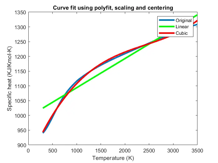
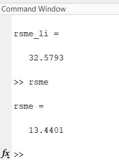
The Root Mean Square Error (RSME) of the Linear and Cubic polynomial fit with respect to the original data using this method is therefore 32.6 and 13.4, respectively.

Fitness of this cubic curve:

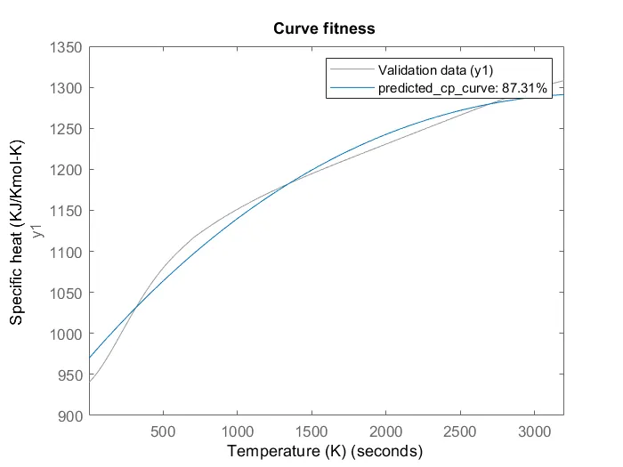
The fitness of this cubic polynomial curve is therefore 87.31%.

IV.1.3. CODE EXPLANATION:

1. The data file is loaded into a celled matrix variable called data
2. The data is segregated into their respective sections. Temperature - x-axis and Specific heat y-axis.
3. The temperature data is normalized with the help of scaling and centring to condition the nth degree polynomial. n is greater than 2.
4. The coefficient of the linear polynomial is generated and put into co_effs_linear variable using the polyfit command.
5. Now the value of cp for the linear curve is predicted using the polyval command by inputting the coefficient and the normalized temperature values.
6. Now the coefficients of the cubic polynomial is calculated using the polyfit command and put into the co_effs matrix.
7. Then the values of cp for the cubic polynomial curve is predicted using the polyval command and put into the predicted_cp matrix.
8. Calculating the root mean square error
   1. Error = actual data - predicted data
   2. The error is squared
   3. The mean square error is the mean of all the square errors obtained
   4. The root mean square error is, therefore, the square root of the mean square error.
   5. The values is put in the rsme variable.
9. Now the graphs are plotted, comparing the original data to the predicted data.
10. Finally, curve fitness is calculated
    1. Identify the 3rd order polynomial with the help of ssest() command.
    2. compare the predicted data to the original data with the help of compare() command.
    3. The graph will be plotted along with the fitness value printed on the legend.

IV.2. MATLAB CODE USING SPLIT-WISE METHOD

clear all
close all
clc

data = load('data'); % Copy the data of data file into data array

% Segrigating the data
temp_data = data(:,1)'; % Temperature values
cp_data = data(:,2)'; % Specific heat values
plot(temp_data,cp_data,'Color','b','Linewidth',2)
hold on

% Scaling and centering the x-axis variables which is the temperature here
temp_scale = normalize(temp_data,'scale'); % Scaling
temp_norm = normalize(temp_scale,'center','mean'); % Centering

b = 4; % Number of splits
N = numel(temp_norm);
x = N*ones(1,b)/b; % Array creater
temp = mat2cell(temp_norm,1,x); %Converting the temp_data matrix into 4 by cell
cp = mat2cell(cp_data,1,x); % Converting the cp_data matrix into 4 by cell
p_cp = mat2cell(cp_data,1,x); % Initiating the p_cp array

for i = (1:b)
    co_effs = polyfit(temp{i},cp{i},3); % Coefficient values to generate a cubic curve fit
    p_cp{i} = polyval(co_effs, temp{i}); % Predectited speacific heat values
end

predicted_cp = cell2mat(p_cp);

% Calculating the Root Mean Squared Error (RMSE)
% Calculating the Square error = error^2; error = original - produced data
for i = (1:length(cp_data))
    sq_error = (cp_data(i) - predicted_cp(i))^2;
end

% Calculating the Mean Square error = Average of Square error
mse = sum(sq_error)/length(sq_error);

% Root mean square error = mse^0.5
rsme = mse^0.5;

figure()
plot(temp_data,cp_data,'Color','b','Linewidth',2) % PLotting the orignal data in blue
hold on
plot(temp_data,predicted_cp,'Color','r','Linewidth',2) % PLotting the predicted data in red
title('Curve fit using splitwise, polyfit, scaling and centering')
xlabel('Temperature (K)')
ylabel('Specific heat (KJ/Kmol-K)')
legend('Original','Cubic')

% Curve fitness
predicted_cp_curve = ssest(predicted_cp',3); % identifying a 3rd order curve
figure()
compare(cp_data',predicted_cp_curve) % Using the compare command to simulate the sys response and plot it alongside the data cp_data.
title('Curve fitness with split-wise method')
xlabel('Temperature (K)')
ylabel('Specific heat (KJ/Kmol-K)')

IV.2.1. RESULTS:

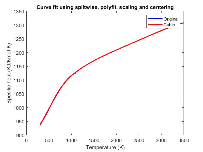
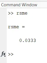
The Root Mean Square Error (RSME) of the Cubic polynomial fit with respect to the original data using this split-wise method is therefore equal to 0.0333.

Fitness of this cubic curve:

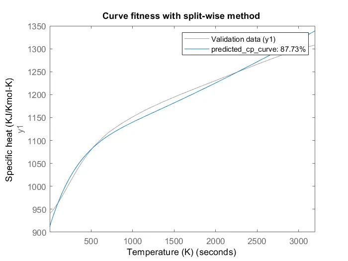
The fitness of this cubic polynomial curve derived by using split-wise is therefore 87.73%.

IV.2.3. CODE EXPLANATION:

1. The data file is loaded into a celled matrix variable called data
2. The data is segregated into their respective sections. Temperature - x-axis and Specific heat y-axis.
3. The temperature data is normalized with the help of scaling and centering to condition the nth degree polynomial. n is greater than 2.
4. Now splitting the data (temp, cp) into 4 equal sections aka split-wise method, I am using the mat2cell command to do that, later which will need to be converted back using cell2mat for plotting purposes.
5. Now the coefficients are calculated with the polyfit() command within the loop which will run for the number of splits we made. Also, the predicted specific heat values are calculated within the loop.
6. Now the predicted cp matrix which has 4 cells is converted bank into a 1-by matrix using the cell2mat as discussed earlier.
7. Calculating the root mean square error
   1. Error = actual data - predicted data
   2. The error is squared
   3. The mean square error is the mean of all the square errors obtained
   4. The root mean square error is, therefore, the square root of the mean square error.
   5. The values is put in the rsme variable.
8. Now the graphs are plotted, comparing the original data to the predicted data.
9. Finally, curve fitness is calculated
   1. Identify the 3rd order polynomial with the help of ssest() command.
   2. compare the predicted data to the original data with the help of compare() command.
   3. The graph will be plotted along with the fitness value printed on the legend.

V. ERRORS OR WARNINGS FACED DURING THE CODE

Warning: "Polynomial is badly conditioned."

Solution: It is always recommended to normalize the independent variable (x-axis temperature) with the help of centering and scaling before proceeding to curve fit using polyfit command.

VI. ASSIGNMENT QUESTIONS

1. How to make a curve fit perfectly?

When the root mean square error (RSME) is equal to zero, then the perfect fit is achieved. In order to achieve this, we need to bring in other constraints which the dependent variable depends on other than the x-axis variable. Take our specific heat for example, it not only depends on temperature but also on its mass and heat energy of the substance. the formula for specific heat is `c = Q/(m triangleT)` where Q is the heat energy, m is the mass and `triangleT` is the change in temperature. Employing this into the polynomial function will create the perfect fit with zero errors.

2. How to get the best fit? Note: Best fit and a perfect fit are two completely different phenomena.

The best fit can be achieved by following the below mentioned:

1. Increasing the degree of the polynomial

2. By normalizing i.e., centering and scaling the independent variable (x-axis)

3. By employing the split-wise method and splitting them as many as possible

4. By minimizing error

By using the above methods, we can achieve the root mean square error close to zero. Hence achieving the best fit.

3. What could be done to improve the cubic fit?

A cubic fit can be improved by using the split-wise method along with normalizing (scaling and centering) the x-axis or the independent variable. It can be clearly noted from the above two results that the Root Mean Square Error (RSME) for the curve fit used split-wise was far accurate compared with the later for the same degree of the polynomial.

VII. REFERENCES

1. Mean Square error
2. Polyfit help matlab
3. Compare help matlab
4. Scaling the data