PACJECKA MAGIC TIRE MODEL USING MATLAB
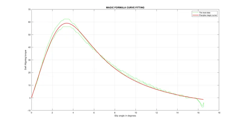
This project aims at using the magic tire formulation to obtain the fit coefficients so that the predicted curve describes the tire test data accurately with a root mean square error of less than 2.0 Nm.
The Pacjecka magic tire model is the most commonly used empirical tire model in practice. It is based on the magic formula below.
The magic formula:
`F_y = D*sin{C*tan^-1[Bx_m-E(Bx_m-tan^-1(Bx_m))]}*mu*Fz`
where `x_m` is the tire slip angle, `mu` is the tire-road friction coefficient, `Fz` is the vertical force and B, C, D and E are fit parameters.
`F_y` is the cornering force, braking force or self-aligning moment
This formula cannot be derived from any first principles. That's why it's called the magic formula. It just has proven to be a very good approximation in many practical applications.
To use this magic formula, we first collect a bunch of empirical data points which is from a plot between the tire slip angle and the ratio of the lateral tire force and the vertical tire force. Then we would fit the model parameters B, C, D & E such that the magic formula curve fits the empirical data points with the least root mean square error.
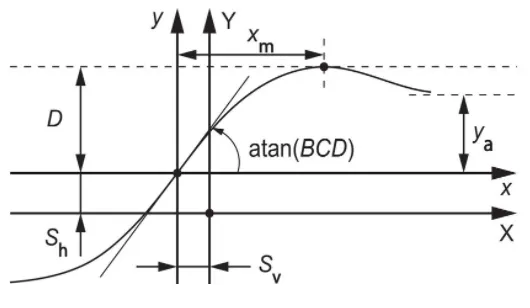
`S_v` and `S_h` are the vertical and horizontal shifts respectively. (Offsets to account for camber thrust, conicity, ply steer or rolling resistance)
The model parameters:
1. B: Stiffness factor - Controls the slope of the magic formula around the origin.
2. C: Shape factor - Controls the location of the peak along the `alpha`-axis.
- C = 1.3 (Lateral force)
- C = 1.65 (Longitudinal force)
- C = 2.4 (Self-aligning force)
3. D: Peak value - Controls the height of the peak.
4. E: Curvature factor - Controls the shape of the peak.
- `E = (Bx_m-tan(pi/(2C)))/(Bx_m - tan^-1(Bx_m)`
Aim:
To perform curve fitting using Pacjeka magic formula.
Inputs:
Tire test data: Composed of Slip angles and Aligning torque values derived from the tire test.
Matlab Code:
close all
clear all
clc

data = load('tire_test_data');
a = data(:,1);
Mz = data(:,2);

% Model parametres
B = 0.2;
C = 2.18;
D = 59;
E = -2.5;
Sh = 0;
Sv = 0;

% Test data model
MZ_data = zeros();
for j = 1:length(Mz)
    MZ_data(j) = D*sin(C*atan(B*a(j)-E*(B*a(j)-atan(B*a(j)))))+Sv;
end

% Pacejka's model
A = zeros(); MZ = zeros(); sq_error = zeros();
xm = linspace(0,100,length(Mz));
for i = 1:length(Mz)
    A(i) = Sh + xm(i)*0.165;
    MZ(i) = D*sin(C*atan(B*A(i)-E*(B*A(i)-atan(B*A(i)))))+Sv;
    % Square Error
    sq_error(i) = (MZ_data(i)-MZ(i))^2;
end

% Root mean squared error
rms = sqrt(sum(sq_error)/length(sq_error));
fprintf('The Root mean square error is %0.3f',rms);

% Plot
figure()
plot(a,Mz,'Color','g')
xlabel('Slip angle in degrees')
ylabel('Self Aligning torque')
grid on
hold on
plot(A,MZ,'Linewidth',1.5,'Color','r')
title('MAGIC FORMULA CURVE FITTING')
legend('Tire test data','Pacejka magic curve')
RMS Value:

The root mean square error (RMS) is 1.961 Nm, which is less than 2 Nm. Hence passing the quality standard for this test.
Plots:
References: