Damped simple pendulum ODE simulation using Matlab

SIMPLE PENDULUM

A simple pendulum consists of a heavy point mass suspended from rigid support by means of an elastic inextensible string. The motion of a simple pendulum without damping is like simple harmonic motion and the angular displacement is given by,

`theta = theta_maxsinroot2 (g/L)t`

where,

`theta` is the angular displacement of the pendulum at time t

`theta_max` is the maximum angular displacement of the pendulum

g is the acceleration due to gravity

The period of motion T is given by,

`T = 2pi root2 (L/g)`

DAMPING & DAMPING COEFFICIENT

Any influence that tends to dissipate the energy of the system by any form of resistance is called damping. The Damping coefficient is the coefficient of proportionality between the damping force and relative velocity.

`b = 2epsilonroot2 (mk)`

where,

`b` is the damping coefficient

`epsilon` is the damping factor

`m` is the mass

`k` is the equivalent force constant

• if `epsilon` = 1, the damping is known as a critical damping condition.
• if `epsilon` > 1, the system is overdamped. In practice, no mechanical systems have over damping.
• if `epsilon` < 1, the system is underdamped.

ORDINARY DIFFERENTIAL EQUATIONS

An ordinary differential equation is an equation that contains one or more functions and derivatives of only one independent variable. An ODE of order n is an equation of the form `F = (x,y,y',......,y^n) = 0`, where x is the independent variable, `y` is a function of `x`, `y' = dy/dx` is the first-order derivative and `y^('n) = (d^ny)/dx^n` is the `n^(th)` order derivative.

ODE OF A DAMPED SIMPLE PENDULUM

The ordinary differential equation which describes the motion kinematic of a damped simple pendulum is given below.

`(d^2theta)/dt^2 + b/m(d theta)/dt + g/L sintheta = 0` --------------------------------- eqn.(1)

The same equation can also be used for a spring, mass and damper system. This has a lot of applications in vehicle dynamics where the suspension system can be modelled using this differential equation.

For converting the 2nd order ODE to 1st order ODE,

Let `theta = theta_1`,

Then,

`=> (d theta)/dt = (d theta_2)/dt = theta_2` ---------------------------------- eqn.(2)

`=> (d^2theta)/dt^2 = (d^2theta_1)/dt^2 = d/dt[(d theta_1)/dt] = (d theta_2)/dt` ------------------------------- eqn.(3)

So, the equation 2 is converted to a first order differential equation as follows.

`(d theta_2)/dt + b/m theta_2 + g/L sintheta_1 = 0` ----------------------------------- eqn.(4)

`=> (d theta_2)/dt = -b/m theta_2 - g/L sintheta_1` ---------------------------------- eqn. (5)

`=> (d theta_1)/dt = theta_2`

I. AIM

To write a program that solves the equation of motion of a simple pendulum with damping.

II. OBJECTIVES

• To generate the Angular displacement & velocity vs time plot
• To simulate the motion of the simple pendulum

IV. MATLAB CODE

IV.1. SIMPLE PENDULUM SIMULATION CODE:

% Input values

L = 1; % Radius of Pendulum arc in m
m = 1; % Mass of pendulum in kg
b = 0.05; % Damping coefficient
g = 9.81; % Acceleration due to gravity m/s^2

% Conditions
in_ang_disp = 0; % Initial angular displacement
in_ang_v = 3; % Initial angular velocity in radians/s

theta_0 = [in_ang_disp;in_ang_v];

t_span = 20; % Total time of video in seconds
fps = 30; % Frames per second
t_pts = linspace(0,t_span,fps*t_span); % Time points for t_span seconds

% ODE Solver
[t, results] = ode45(@(t,theta) simp_pend_ode_func(L,theta,b,g,m),t_pts,theta_0);

ang_disps = results(:,1); % Angular displacement array
ang_vs = results(:,2); % Angular velocity array

% Fixed point of the pendulum
x0 = 0; % x origin coordinate
y0 = 0; % y origin coordinate

ct = 1; % Counter for counting the total number of frames

% Pendulum ball dimensions
r = 0.1; % Radius in m

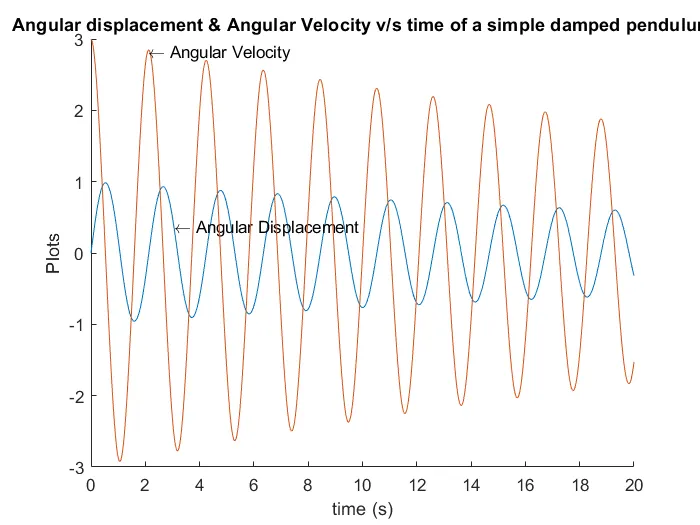
% Angular displacement & Angular velocity v/s time plot

figure()
hold on
title("Angular displacement & Angular Velocity v/s time of a simple damped pendulum")
plot(t,ang_disps)
text(3.052,0.3727,'leftarrow Angular Displacement')
plot(t,ang_vs)
text(2.088,2.83,'leftarrow Angular Velocity ')
ylabel('Plots')
xlabel('time (s)')

% The animation loop

figure()
for i = 1:length(t_pts)
    pos = ang_disps(i); % Angular displacement of pendulum at a point of time
    
    y = -L*cos(pos); % x coordinate of pendulum at a point of time
    x = -L*sin(pos); % y coordinate of pendulum at a point of time
        
    % Animation plots
    
    plot([x0 x],[y0 y],'linewidth',3,'Marker','O','Markersize',15,'MarkerFaceColor','r','MarkerEdgeColor','r') % The pendulum plot
    axis([-1.5 1.5 -1.5 1.5]) % Axis of the plot
    
    rectangle('Position',[-1.5 0 3 0.5],'Facecolor',[0.2 0 0],'Edgecolor',[0 0 0])

    pause(t(2)) % Determines the time b/w the frames Also, t(2) = 1/fps
    M(ct) = getframe(gcf);
    ct = ct+1; % Counter gets incremented after the frame is collected
end

% The movie

movie(M);
videofile = VideoWriter('simple_pendulum.avi','Uncompressed AVI'); % Naming and formating the video
open(videofile) % Open the video editor
writeVideo(videofile,M) % Convert the image to frame
close(videofile) % Close the video writer

IV.2. ODE FUNCTION CODE:

function [dtheta_dt] = simp_pend_ode_func(L,theta,b,g,m)
    theta1 = theta(1); % Theta 1 = 1st column of theta
    theta2 = theta(2); % Theta 2 = 2nd column of theta
    dtheta1_dt = theta2; % dtheta1/dt = theta2
    dtheta2_dt = -(b/m)*theta2 - (g/L)*sin(theta1); 
    dtheta_dt = [dtheta1_dt; dtheta2_dt]; % t, angular displacements and angular velocities
end

V. OUTPUTS

V.1. PLOTS:

V.2. SIMULATION:

VI. STEPWISE CODE EXPLANATION

VI.1. MAIN CODE

1. The values of length, mass, damping coefficient and acceleration due to gravity are inputted.
2. The initial angular displacement and angular velocity are set and are fed to theta_0 in a column-wise manner.
3. The time of simulation (t_span), frames per second (fps) are set and the total number of time points (t_pts) is equal to the product of t_span and fps.
4. All the above values are then fed to the ode45 function which would then solve the ODE. And the explanation of this function is in section V.2.
5. This function released three-column arrays t array hold time and the results array holds angular displacements and angular velocities, respectively.
6. The first part of the results array is stored in ang_disps and the later in ang_vs.
7. The fixed point of the pendulum is set to origin coordinates (0,0).
8. The counter ct is initiated at 1
9. The Angular displacement & velocity v/s time plot is now plotted.
10. The loop for stacking up the generated frames is now initiated using for loop.
    1. The loop will run t_pts number of times
    2. For each point in t_pts, co-ordinates x and y are calculated.
    3. For each point in t_pts, the pendulum position is plotted on the graph
    4. To set the pace of the video, the code stops for a duration of 1/fps seconds.
       • For a 30fps video, It should take t_span seconds to generate t_pts plots.
       • So, it takes t_span/t_pts = 1/fps seconds to generate 1 plot.
    5. The getframe(gcf) command collects the current plot and converts it into Matlab image and along the loop feeds it into incrementing positions in the M(ct) array.
    6. The counter ct is incremented by 1
    7. After finishing t_pts times of loop, it finally ends
11. Now the array M(ct) containing the MatLab images of the t_pts number of plots, are converted into frames and stitched together using the movie(M) function.
12. After formatting and writing the video, the video writer closes and saves the video.

VI.2. ODE FUNCTION CODE

1. The function is initiated with dtheta_ft as the output and is dependent on the Length, initial angular displacement, angular velocity, damping coefficient, acceleration due to gravity and mass.
2. As the theta array has two values governed by the eqn.(2) and eqn.(4) are fed to theta1 and theta2 respectively.
3. The calculated values of dtheta1_dt and dtheta2_dt are stored to the output dtheta_dt.
4. The function is ended.

VI.3. ODE45

The ODE45 is an inbuilt MATLAB function that is used to solve Ordinary differential equations. In our case, the syntax is

[t,results] = ode45(@(t,theta) simp_pend_ode_func(L,theta,b,g,m),t_pts,theta_0);

where t and theta are the two inputs to the embedded ode function which we fed it. We also supply tailored values to other inputs such as L,theta,b,g,m,t_pts and theta_0.

The whole function will then put the values into the array [t,results]. Where in results has two sub-arrays supplied from theta in the ode45 function which also has two parts.

It is mandatory to convert the nth order differential equation to convert to 1st order differential equation before feeding it to the ode45 function which the simp_pend_ode_func() takes care of.

VII. ERRORS FACED DURING THE CODE

Problem: When the Angular displacement and angular velocity v/s time plot is placed to run after the for loop is completed, it did not generate the plot! The command windows didn't show any errors either.

Solution: Place the plotting code above the for loop and don't touch the plot until the simulation is complete.