Thermal efficiency and PV plot of an Air standard Otto cycle

THE OTTO CYCLES:

The Otto-cycle is a cycle of thermodynamic processes used by SI (Spark Ignition) IC engines. Petrol powered engines work on the Otto cycle, where the fuel is combusted with the help of a spark. It consists of two reversible adiabatic (Isentropic) and two constant volume processes.

• Process 0-1: Isobaric expansion process (Air-fuel mixture intake stroke)
• Process 1-2: Reversible adiabatic compression of the air-fuel mixture (Isentropic compression)
• Process 2-3: Isochoric heat addition process (Spark ignition/Combustion)
• Process 3-4: Reversible adiabatic expansion of combustion mixture (Power stroke)
• Process 4-1: Isochoric heat rejection process (Exhaust)

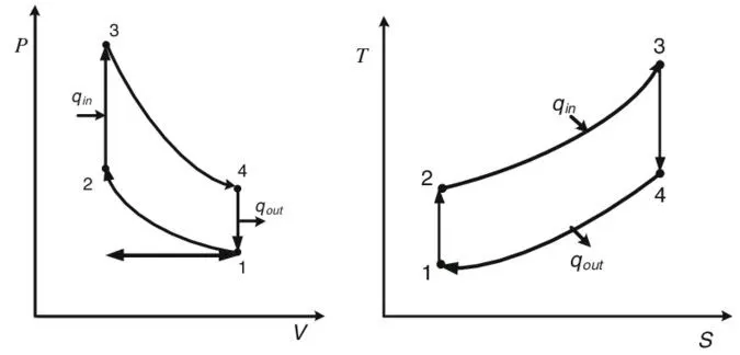
Image description: Example of the PV and TS plots of an ideal Otto cycle.

VOLUME TRACE:

`V = [1+(cr-1)/2*(R + 1 - cos(theta) - (R^2 - sin^2(theta))^(1/2))*V_c`

where,

V = Volume trace

`R = 2*(controd)/(stroke)`

cr = Compression ratio

Vc = Clearance volume

THERMAL EFFICIENCY OF THE OTTO CYCLE:

The thermal efficiency of an otto cycle is the ratio of heat supplied and the heat rejected during the isochoric processes.

`Thermal Efficiency = (Qi - Qo)/(Qi)` => `1 - (T1)/(T2)` => `1-1/(r^(y-1)`

Where,

Qi is the heat supplied during the Isochoric heat addition process (Spark ignition)

Qo is the heat rejected during the Isochoric heat rejection process (Exhaust)

T1 and T2 are the temperatures at state 1 and 2 respectively

r is the Compression ratio

y is the ratio of specific heat, which is 1.4 for air.

I. AIM:

To write a MATLAB code that can solve an otto cycle and make plots for it.

II. OBJECTIVES:

1. Create a PV diagram of the otto cycle
2. Calculate the thermal efficiency of the otto cycle

IV. THE CODE:

IV.1. OTTO-CYCLE MATLAB CODE

gama = 1.4; % Ratio of specific heat for air

% Engine geometric parameters

bore = 0.1; % Bore diameter in meters
stroke = 0.1; % Length of stroke in meters
cont_rod = 0.15; % Length of connecting rod in meters
cr = 12; % Compression ratio

% Calculating the swept volume and the clearance volume

swept_vol = (pi*stroke/4)*bore^2; % Swept volume in m^3
clear_vol = swept_vol/(cr-1); % Clearance volume in m^3

% State 1 Variables

p1 = 101325;
t1 = 500;
v1 = swept_vol + clear_vol; % Volume at state 1

% State variables at state point 2

v2 = clear_vol; % Volume at state 2

% p2 x v2^gama = p1 x v1^gama
% p2 = p1 x (v1/v2)^gama = p1 x cr^gama
p2 = p1*cr^gama; % Pressure at state 2

% p1 x v1 / t1 = p2 x v2 / t2 => t2 = p2 x v2 x t1 / (p1 x v1)
t2 = p2*v2*t1/(p1*v1); % Temperature at state 2

% State variables at state 3

v3 = v2; % Volume at state 3
t3 = 2300; % Temperature at state 3
p3 = p2*t3/t2; % Pressure at state 3

% State variables at state 4

v4 = v1; % Volume at state 4
p4 = p3*(v3/v4)^gama; % Pressure at state 4
t4 = p4*v4*t3/(p3*v3); % Temperature at state 4

% Thermal efficiency of an otto cycle
% Thermal effieciency = (Qin - Qout)/Qin => 1 - (t1/t2) = 1 - 1/cr^(gama-1)
ther_eff = 1 - 1/cr^(gama-1); 

% Piston Kinematics for Icentropic compression process

c = p1*v1^gama;
v_compression = engine_kinematics(stroke,cont_rod,cr,180,0,clear_vol);
p_compression = c./v_compression.^gama;

% Piston kinematics for the isentropic expansion process

c = p3*v3^gama;
v_expansion = engine_kinematics(stroke,cont_rod,cr,0,180,clear_vol);
p_expansion = c./v_expansion.^gama;

% Plotting the pv diagram
figure()
hold on
title("Pressure v/s Volume plot of an Ottocycle")
xlabel("Volume (m^3)")
ylabel("Pressure (pa)")
plot(v2,p1,"*","Color",'r')
text(v2,p1,'leftarrow 0')
plot(v1,p1,"*","Color",'r')
text(v1,p1,'leftarrow 1')
plot(v_compression,p_compression)
text(0.0001325,2353000,'leftarrow Isentropic expansion process')
plot(v2,p2,"*","Color",'r')
text(v2,p2,'leftarrow 2')
plot(v3,p3,"*","Color",'r')
text(v3,p3,'leftarrow 3')
plot(v_expansion,p_expansion)
text(0.0001755,932700,'leftarrow Isentropic compression process')
plot(v4,p4,"*","Color",'r')
text(v4,p4,'leftarrow 4')
plot([v1 v2],[p1 p1])
plot([v2 v3],[p2 p3])
text(6.75^-05,4000000,'leftarrow Constant volume heat addition process')
plot([v1 v4],[p1 p4])
grid on

IV.2. ENGINE KINEMATICS FUNCTION CODE:

function [V] = engine_kinematics(stroke,cont_rod,cr,start_crank,end_crank,clear_vol)
    % Start_crank is the angualar position of flywheel when the piston is at the top dead centre
    % End_crank is the angular position of flywheel when the piston is at
    % the bottom dead centre
    theta = linspace(start_crank,end_crank,180); 
    
    R = 2*cont_rod/stroke; % Assembly height
    
    % Calculation of the Volume trace
    term1 = 0.5*(cr-1);
    term2 = R + 1 - cosd(theta);
    term3 = (R^2 - sind(theta).^2).^0.5;
    V = (1 + term1*(term2 - term3)).*clear_vol; % Volume trace in m^3
end

V. OUTPUTS:

V.1. PV Plot of the Otto cycle

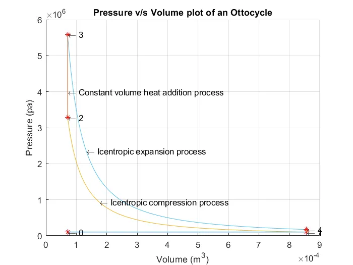
Output description: (Missing information)

• Process 0-1: Intake stroke
• Process 4-1: Isochoric heat rejection process (Exhaust)

V.2. Thermal Efficiency of the Otto cycle:

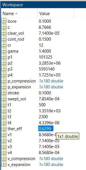
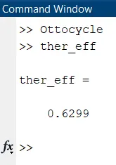
The thermal efficiency of this otto cycle is 62.99%.

VI. STEPWISE CODE EXPLANATION

1. MAIN CODE

1. The code is stared with feeding the values of the ratio of specific heat (y) (1.4 for air) and engine geometric parameters- Bore, stroke, length of connecting rod and the compression ratio (cr).
2. Now, the swept volume and the clearance volume is calculated by inputting the parameters.
   1. Swept volume = `pi/4*STROKE*(BORE )^2`
   2. Clearance volume = `(swept volume )/ (compression ratio -1)`
3. Now the state properties at 1 are determined. The pressure and volume at this state are already known so the values are directly inputted. The volume is equal to the sum of swept volume and clearance volume.
   1. Volume at state 1 = Swept volume + Clearance volume
4. The volume at state 2 is equal to the clearance volume. The values of pressure p2 and temperature t2 at this state needs to be derived.
   1. `p_2 * v_2^y = p_1 * v_1^y => p_2 = p_1*(v_1/v_2)^y = p_1*cr^y`
   2. `t_2 = (p_2*v_2*t_1)/(p_1*v_1)`
5. The volume at state 3 is equal to the volume at state 2 (Isochoric heat addition process), the temperature is at 2300k and p3 needs to be calculated.
   1. `p_3 = p_2*t_3/t_2`
6. The volume at state 4 is equal to the volume at state 1. The values of pressure and temperature needs to be calculated.
   1. `p_4 = p_3*(v_3/v_4)^y`
   2. `t_4 = (p_4*v_4*t_3)/(p_3*v_3)`
7. After obtaining all the property values at the 4 states of the otto cycle, now we can calculate the thermal efficiency of the cycle. The explanation of this is explained at the theory part of this report.
   1. Thermal efficiency = `1 - (1/(cr^(y-1)))`
8. For calculating pressure trace, we need to determine the constant for reversible adiabatic compression and expansion.
   1. constant of reversible adiabatic compression = `p_1*v_1^y`
   2. constant of reversible adiabatic expansion = `p_3*v_3^y`
9. Now the volume trace for reversible adiabatic compression and expansion is obtained by using the engine kinematics function which will be discussed in the next section.
10. Pressure traces:
    1. Pressure trace of adiabatic compression = adiabatic const/compression volume trace^y
    2. Pressure trace of adiabatic expansion = adiabatic const/expansion volume trace^y
11. Now the PV graph of the otto cycle is plotted.

2. ENGINE KINEMATICS CODE

1. First, the function is defined by giving it the name "engine_kinematics" and V (volume trace) as the output of the function. And including the stroke, connecting rod length, start crank, end crank and the clearance volume as the function parameters.
   
2. The angles of flywheels are defined as 180 angles between the start crank and the end crank.
3. Now the assembly height (R) is calculated
   1. `R = (2*conrod)/(stroke)`
4. Since the formula for the volume trace is big, it would become a bit tedious to frame the expression in Matlab as a whole. So I am doing it in parts.
   1. term 1 = `0.5*(cr-1)`
   2. term 2 = `R + 1 - cos(theta)`
   3. term 3 = `(R^2 - sin(theta)^2)^(1/2)`
   4. Volume trace = [1 + term1*(term2 - term3)]*clearance volume

VII. ERRORS FACED DURING THE PROJECT

Issue: The linspace command was syntaxed incorrectly in the engine kinematics function code due to which the function was not executing and hence the volume traces were not getting plotted. Even the command window was not showing it.

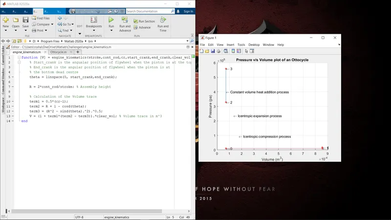
Solution: Re-syntaxed the linspace command and the plots were visible.