Steady Vs Unsteady flow over a cylinder
Steady Vs Unsteady flow over a cylinder
Objectives : 1. To simulate the flow over a cylinder in steady state for Reynolds number (Re) ranging from 10 - 1,00,000.
2. To simulate the flow over a cylinder for transient condition at Re 100 and calculate the Strouhal number(St).
Theory :
A cylinder is a bluff body, which restricts the flow over it and has a high coefficient of drag. The flow over a cylinder is important because it experiences a boundary layer separation and periodic oscillations of flow in the wake region behind the cylinder[1].
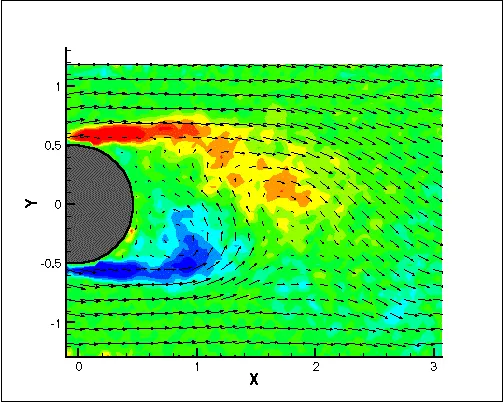
Fig .1 : Periodic oscillations and vortex shedding in the wake of the cylnder
In a particular reynolds number range, a oeriodic flow develops in the wake of the cylinder as a result of boundary layer vortex being shed alternatively from either side of the cylinder. This regular pattern of vortices in the wake is called Karman vortex street.
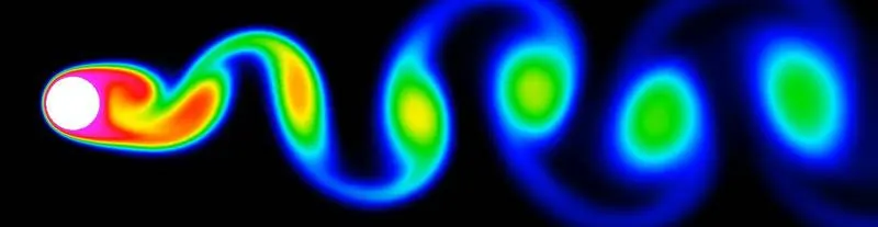
Fig.2 : Karman vortex street visualization using Vislt, an open source CFD post processing tool [2].
The periodic nature of the vortex shedding phenomenon can sometimes lead to unwanted structural vibrations, especially when the shedding frequency matches one of the resonant frequencies of the structure.
Flow over a cylinder simulation using ANSYS FLUENT :
Step.1 : Geometry creation
Launch the ANSYS Workbench and create a ANSYS FLUENT project in the project schematic window of Workbench.
Now, double click on the SpaceClaim tool. When the Modelling software window opens switch from the isometric view to Top view.
Using the Circle option in the draw tool bar, create a circle of diameter 2m. Draw a rectangle of length 60m and width 20m which encloses the circle. This rectangle acts as the computational domain.
Using the pull tool highlight the face of the rectangle and then click on the circle and delete the surface of the circle.
Exit the SpaceClaim.
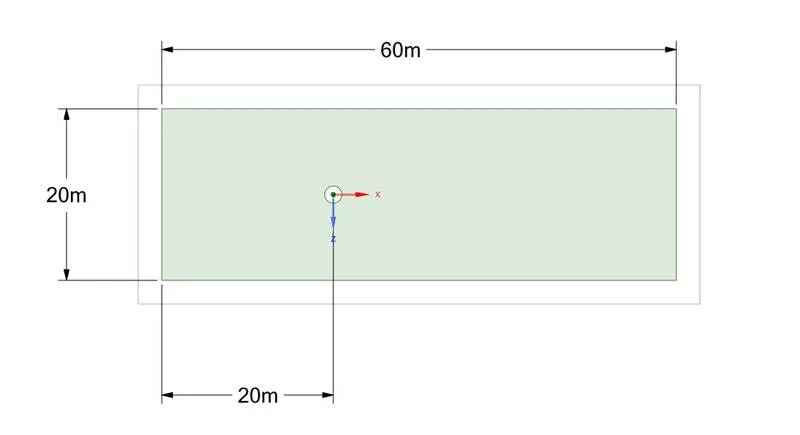
Fig. 3 : Geometry creation in the SpaceClaim
Step.2 : Meshing
Launch the ANSYS Mesher and then name the respective edges as inlet, Outlet, cylinder wall and Symmetry. These serve as the boundary conditions in the FLUENT.
Use the Triangles method for generating the preliminary mesh.
Then using the edge sizing method, divide the perimeter of the circle into 36 divisions. This is to increase the cell count on the boundaries and consequently for better visualization of the flow.
Also use the inflation layers on the perimeter of the circle.
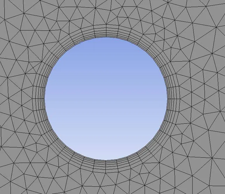
The final mesh should look as follows.
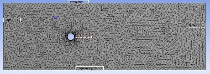
Fig. 4: Final Mesh.
Step. III : Solution setup
a. Steady case :
- As soons as the mesh loads into the setup of the ANSYS FLUENT, check for the quality of the mesh.
- Procced to set the General tab, of the setup and select the steady state simulation.
- Now click on the Models option, and set the viscosity to Laminar.
- Create a user defined material by clicking on the Materials option and set its density as 1 kg/m^3 and Dynamic viscosity as 0.05 Kg/m-s.
- Assign this user created material to the fluid zones by clicking on the cell zone conditions.
- In the boundary conditions option click on the inlet boundary condition. By default this is set to velocity inlet which is the required condition. Input the inlet flow velocity as 0.25 m/s for a Re 10.
The following boundary conditions are set at the respective places :
| Location | Boundary condition | Value |
| Inlet | Velocity inlet |
0.25 m/s for Re 10 2.5 m/s for Re 100 25 m/s for Re 1000 250 m/s for Re 10,0000 2500 m/s for Re 1,00,000 |
| Outlet | Pressure outlet | Gauge pressure |
| Domain walls | Symmetry | No shear stress |
| Cylinder walls | wall | No slip condition for velocity. |
- For the solution methods, use the SIMPLE scheme.
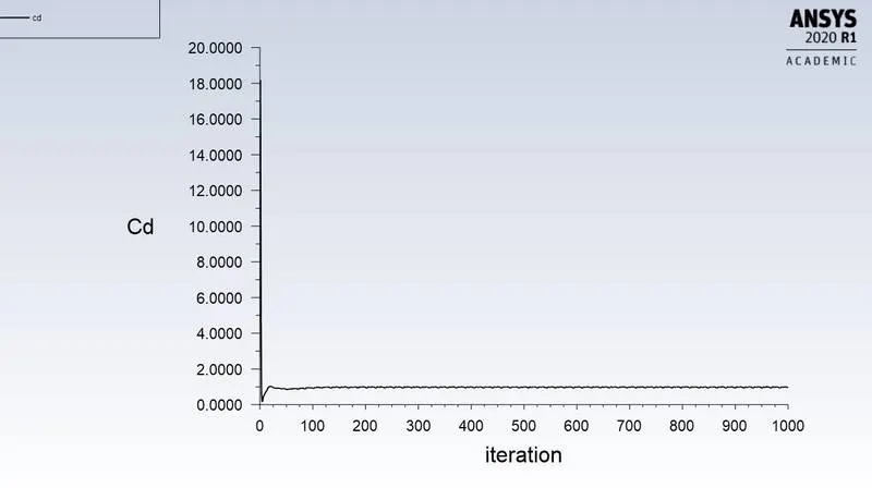
- In the report definition option under the solution tab, create a report definition for Coefficient of drag (Cd) and Coefficient of Lift (Cl) calculated at the cylinder wall.
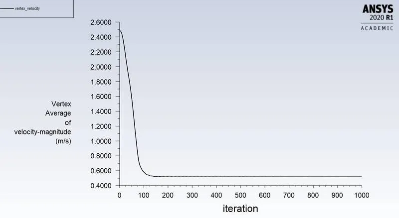
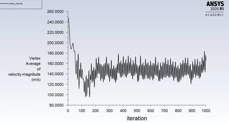
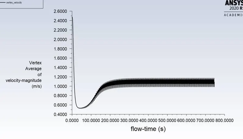
- Create another report definition for Vertex average value of velocity calculated at a point located at a position 10 m downstream the centre of the circle.
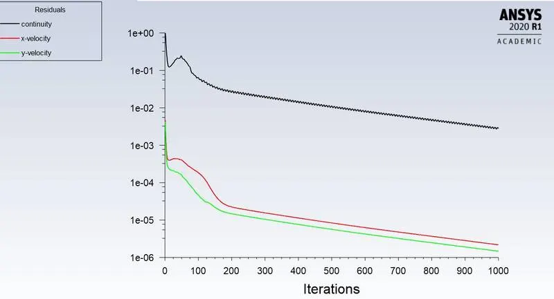
- Initialize the solution using the values at the inlet and run the solver till the convergence is achieved.
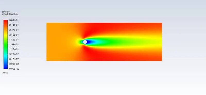
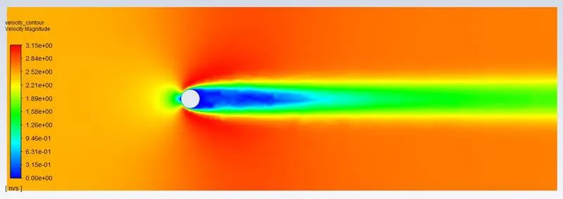
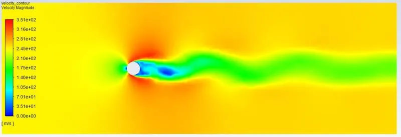
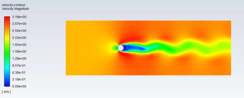
- Finally generate a contour plot for the velocity which shows the vortex shedding phenomenon. Also detremine the value of Cd from the report definition.
b. Transient case
The procedure is same as that of the steady case with an exception that a transient condition is checked instead of steady in the General option under Setup.
Also set desired number of time steps for the solution.
Results :
I. Steady state :
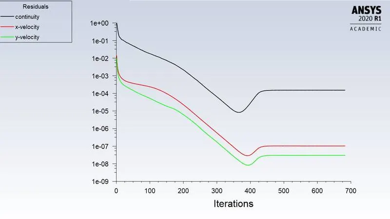
a. For Re 10
Residual plot
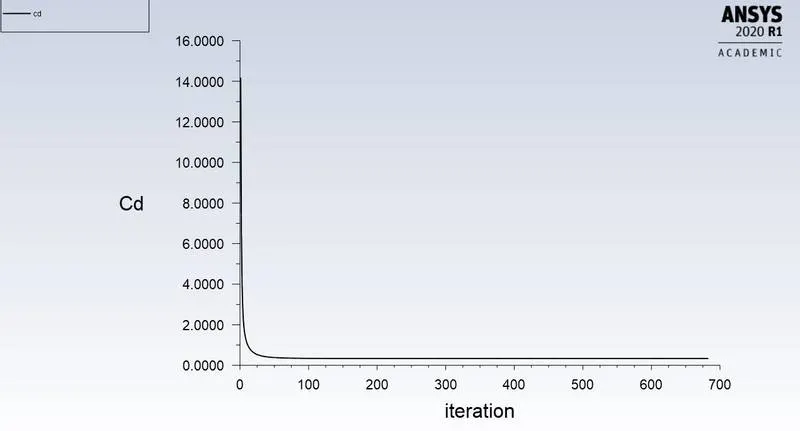
Cd plot
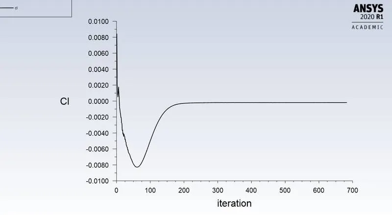
Cl Plot
Velocity contour plot :
b. For Re 100
a. Residual plot
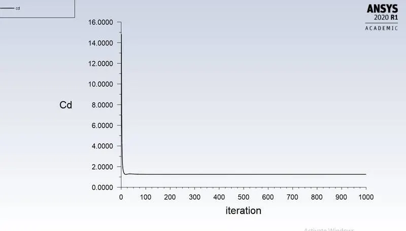
b. Cd plot
c. Cl plot :
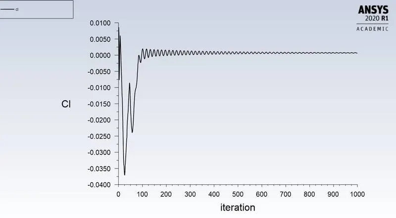
Observation : The fluctuations in the Cl Plot after 120 iterations is due to the periodic oscillations developed at the wake of the cylinder.
d. Vertex average velocity plot :
e. Velocity contour plot
c. For Re 1000
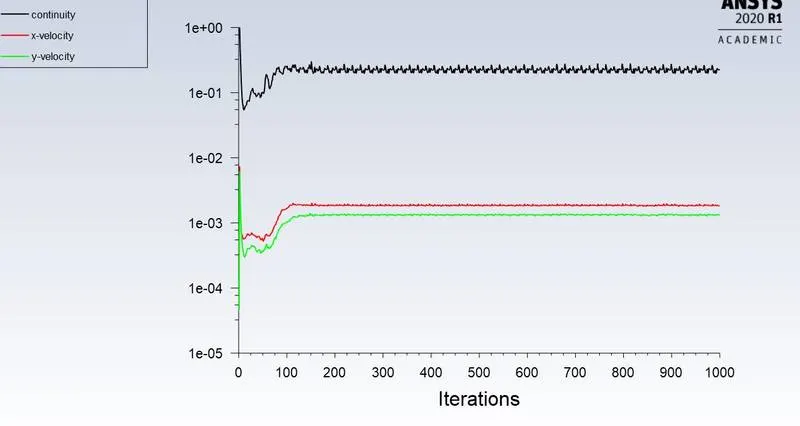
Residual plot
Cd plot
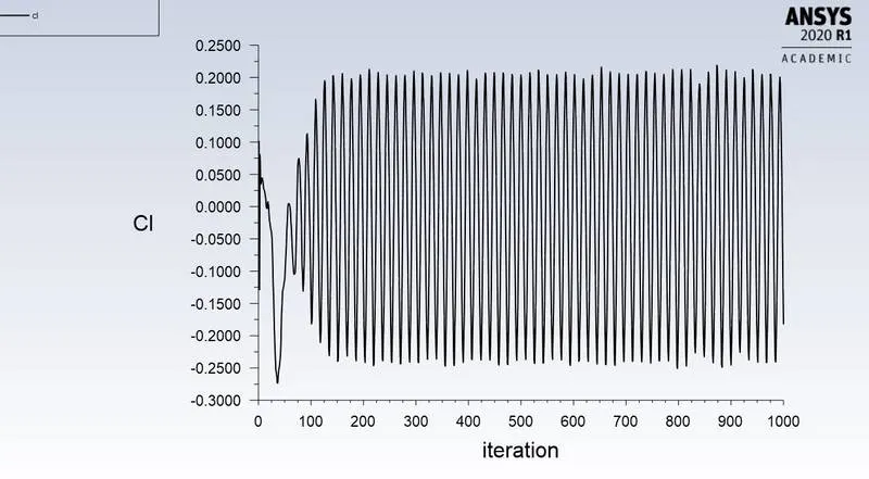
Cl plot:
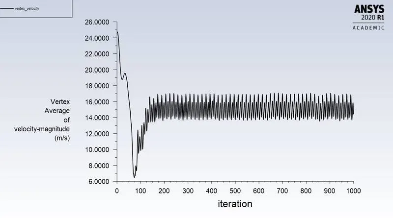
Vertex average velocity plots:
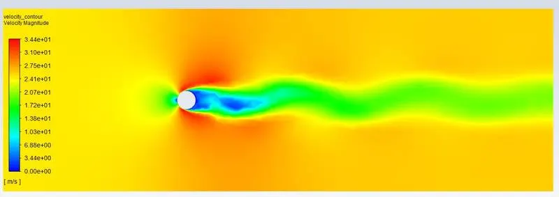
Velocity contour plot :
For Re 10,000
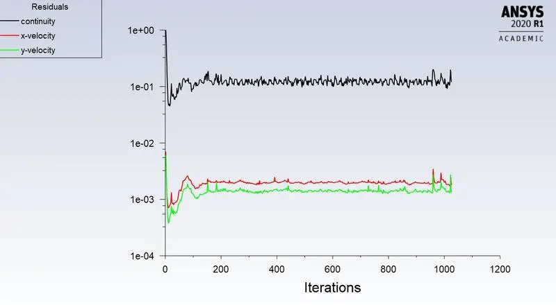
Residual plot :
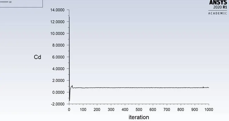
Cd plot :
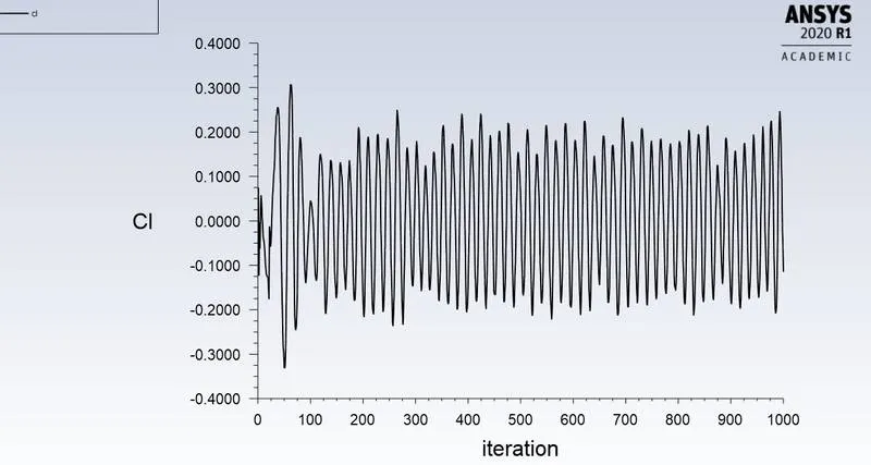
Cl plot :
Vertex average velocity plot :
Velocity contour plots :
For Re 1,00,000
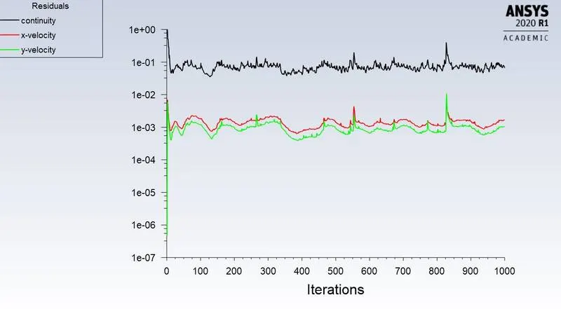
Residual plot
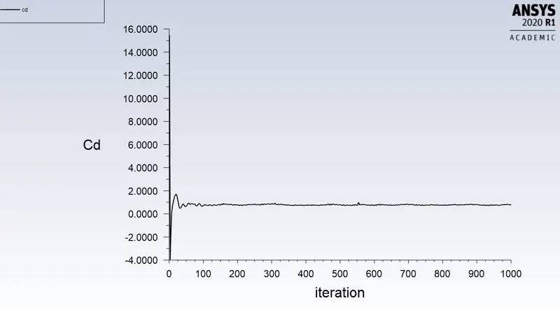
Cd plot:
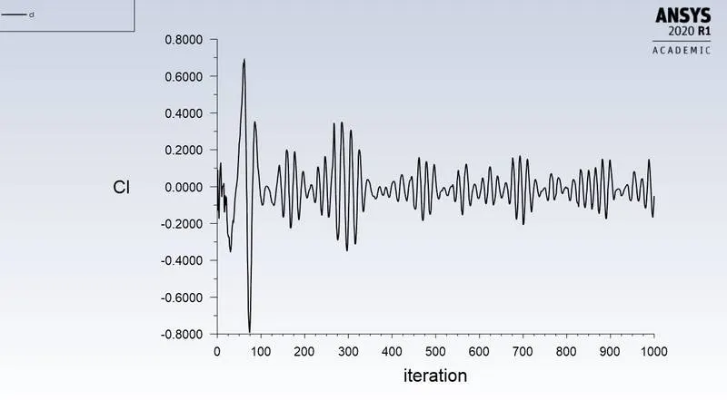
Cl plot :
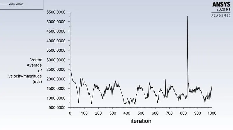
Vertex average values for velocity :
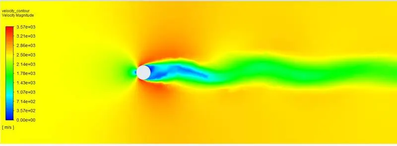
Velocity contour plot :
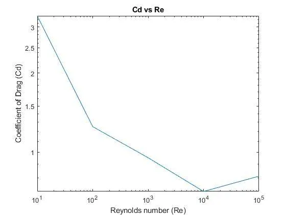
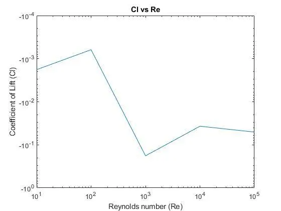
Tabulated values of the Coeffiecient of drag for Re ranging from 10 to 1,00,000
| Reynolds number(Re) | Coefficinet of Drag (Cd) | Coefficinet of Lift(Cl) |
| 10 | 3.305 | -1.8 e -3 |
| 100 | 1.252 | 6.2 e-4 |
| 1000 | 0.9533 | -0.18 |
| 10000 | 0.7094 | -0.037 |
| 100000 | 0.8109 | -0.0506 |
It can be established from the above data that as the Re number increases the Cd decreases. The reason for this is with the increase in the flow velocity the the flow separation phenomenon subsides and hence the reduction of Drag.
An increase in the value of Drag for a Re 1,00,00 could be becuase of high turbulence and adverse effects of flow separation due to instability.
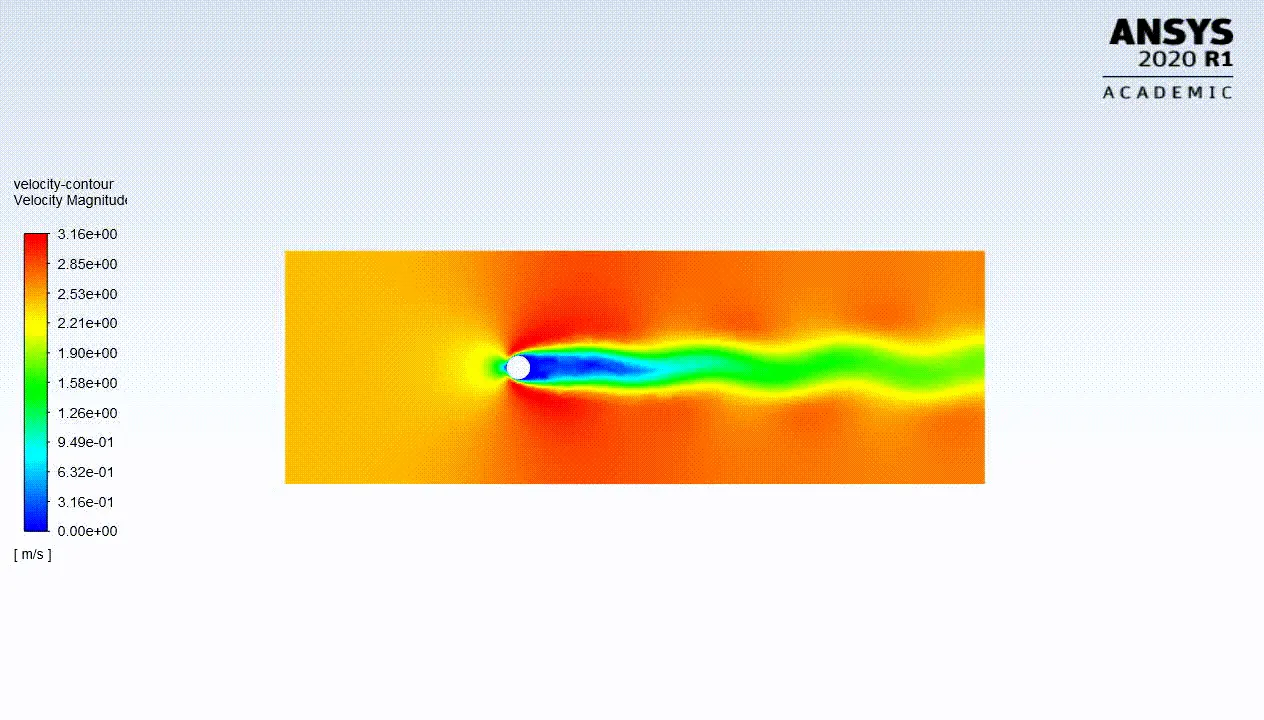
Case II : Transient case
For a Re 100 :
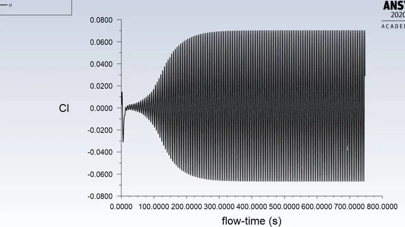
Calculated value of Strouhal number (St) :
St = `f_v * (D/(u))`
`f_v` = 5 / 25 = 0.20
D = cylinder diameter = 2 m.
u = flow velocity = 2.5 m.
Therefore, St = 0.16
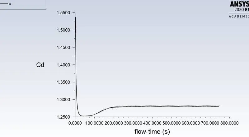
Cd = 1.2814315
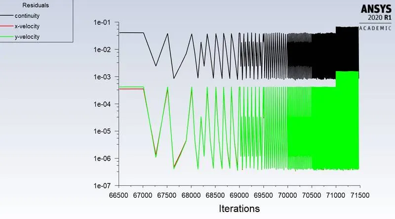
Residual plot :
Cd plot:
Cl plot :
Vertex average velocity plot:
velocity contour plot :
Animation file for the flow over a cylinder :
Preferred material :
A user defined fluid with a density of 1 kg/m^3 and absolute viscosity 0.05 Kg/m-s is chosen for the simultions.
Conclusion :
Flow over a cylinder is simulated for both the steady and unsteady conditions.
Resources :
1. Turbulent wake flow behind the cylinder : http://eng-web1.eng.famu.fsu.edu/~shih/succeed/cylinder/cylinder.htm.
2. Karman votrex street : https://dolfyn.net/dolfyn/gmsh/tutorial08.html