Stability Analysis in Linear System
Week 6 Report.
- Aim: To understand the Stability Analysis in Linear Systems and calculate the Spectral Radius for the different Iterative Methods.
- Theoretical Introduction:
In mathematics, stability theory addresses the stability of solutions of differential equations and of trajectories of dynamical systems under small perturbations of initial conditions. The heat equation, for example, is a stable partial differential equation because small perturbations of initial data lead to small variations in temperature at a later time as a result of the maximum principle. In partial differential equations one may measure the distances between functions using Lp norms or the sup norm, while in differential geometry one may measure the distance between spaces using the Gromov–Hausdorff distance.
In dynamical systems, an orbit is called Lyapunov stable if the forward orbit of any point is in a small enough neighborhood or it stays in a small (but perhaps, larger) neighborhood. Various criteria have been developed to prove stability or instability of an orbit. Under favorable circumstances, the question may be reduced to a well-studied problem involving eigenvalues of matrices. A more general method involves Lyapunov functions. In practice, any one of a number of different stability criteria are applied.
Linear Autonomous Systems:
The stability of fixed points of a system of constant coefficient linear differential equations of first order can be analyzed using the eigenvalues of the corresponding matrix.
An autonomous system
where x(t) ∈ Rn and A is an n×n matrix with real entries, has a constant solution
(In a different language, the origin 0 ∈ Rn is an equilibrium point of the corresponding dynamical system.) This solution is asymptotically stable as t → ∞ ("in the future") if and only if for all eigenvalues λ of A, Re(λ) < 0. Similarly, it is asymptotically stable as t → −∞ ("in the past") if and only if for all eigenvalues λ of A, Re(λ) > 0. If there exists an eigenvalue λ of A with Re(λ) > 0 then the solution is unstable for t → ∞.
Application of this result in practice, in order to decide the stability of the origin for a linear system, is facilitated by the Routh–Hurwitz stability criterion. The eigenvalues of a matrix are the roots of its characteristic polynomial. A polynomial in one variable with real coefficients is called a Hurwitz polynomial if the real parts of all roots are strictly negative. The Routh–Hurwitz theorem implies a characterization of Hurwitz polynomials by means of an algorithm that avoids computing the roots.
Spectral Radius:
In mathematics, the spectral radius of a square matrix or a bounded linear operator is the largest absolute value of its eigenvalues (i.e. supremum among the absolute values of the elements in its spectrum). It is sometimes denoted by ρ(·).
The spectral radius is closely related to the behaviour of the convergence of the power sequence of a matrix; namely, the following theorem holds:
Let A ∈ Cn×n with spectral radius ρ(A). Then ρ(A) < 1 if and only if

- On the other hand, if ρ(A) > 1,
 . The statement holds for any choice of matrix norm on Cn×n.
- Code/Logic:
1. We firstly need to clear and close all the previously entered codes and the present values of the already used variables, hence we use the following commands:
clear all
close all
clc
2. We then start the code by giving all the necessary inputs that are required such as the initial values for x1, x2 and x3. In this case, we will name them as x1_old, x2_old and x3_old respectively.
We must decompose the given co-efficient matrix. We split the matrix into a Lower Diagonal, Upper Diagonal and a Diagonal Matrix to calculate the Iteration Matrix for the three Iterative methods.
Then we must include all the basic inputs, such as the Error value, Tolerance Value and the Relaxation factor as well. The tolerance value used is 1e-4 which is 0.0001 in magnitude. All the inputs are shown below:
x1_old = 0 - Initial Values.
x2_old = 0 - Initial Values.
x3_old = 0 - Initial Values.
L = [0 0 0; -3 0 0; 1 2 0] - %Lower Diagonal Matrix.
U = [0 1 2;0 0 4; 0 0 0] - Upper Diagonal Matrix.
D = [5 0 0; 0 9 0; 0 0 -7] - Diagonal Matrix.
A = L+U+D - Coefficient Matrix.
X = [x1_old; x2_old; x3_old] - Solution Matrix.
B=[10 -14 33] - Residual Matrix.
error = 9e9 - Error Defined.
tol = 1e-4 - Tolerance Defined.
Iterative_solver = [1,2,3] - Defining Iterative Solver array for the for loop.
r = 0.9 - Relaxation Factor.
Jacobian_Iter = 1 - Setting the Iteration counter
GS_Iter = 1 - Setting the Iteration counter
SOR_Iter = 1 - Setting the Iteration counter
I = [1 0 0; 0 1 0; 0 0 1] - Identity Matrix
3. To begin with the logic, we have used a for loop that runs from 1 to the length of all the Iterative solvers. We have created a variable named, Iterative_solvers that has numbers from 1 to 3, because we have three Iterative Solvers to solve from. So, as my loop counter is running from 1 to 3, the Iterative methods will change accordingly as shown in the code.
We must update the values after every iteration so that the code uses the newly calculated values in the nexy iteration.
4. Last but not the least, we must calculate the Eigen Values of Iterative matix for all the Iterative Methods. So, to do this, we have used the command of poly, that will create a Polynomial Function of the given matrix. The syntax for the command is shown below:
p = poly(r)
p = poly(A)
We just extract the roots of this equation and then find the maximum of the absolute of these values. We know that the maximum of all the eigen values is the Spectral Radius of the matrix. If the Spectral Radius of a Matrix is one, it signifies that all the Eigen Values lie in a circle of radius = 1 units.
Main Code:
clear all
close all
clc

%Solving for the given Coefficient matrix

x1_old = 0;                             %Initial Values.
x2_old = 0;                             %Initial Values.
x3_old  = 0;                            %Initial Values.
L = [0 0 0; -3 0 0; 1 2 0];             %Lower Diagonal Matrix.
U = [0 1 2;0 0 4; 0 0 0];               %Upper Diagonal Matrix.
D = [5 0 0; 0 9 0; 0 0 -7];             %Diagonal Matrix.
dm= linspace(0.5,1.5,50);               %Diagonal Magnification Factor
A = L+U+D;                              %Coefficient Matrix.
X = [x1_old; x2_old; x3_old];           %Solution Matrix.
B=[10 -14 33];                          %Residual Matrix.
error = 9e9;                            %Error Defined.
tol = 1e-4;                             %Tolerance Defined.
Iterative_solver = [1,2,3];             %Defining Iterative Solver array for the for loop.
r = 0.9;                                %Relaxation Factor.
I = [1 0 0; 0 1 0; 0 0 1];              %Identity Matrix
Jacobi_Iter = zeros(1,length(dm));      %Setting the Iteration counter
GS_Iter = zeros(1,length(dm));          %Setting the Iteration counter
SOR_Iter = zeros(1,length(dm));         %Setting the Iteration counter


for i=1:length(dm)
D_m = D.*dm(i);

x1_old = 0;
x2_old = 0;
x3_old = 0;
error = 9e9;
%Jacobi Method:
    for e = 1:length(Iterative_solver)

        if Iterative_solver(e) == 1

             while error>tol

                x1 = (10 - x2_old - 2*(x3_old))/(D_m(1,1));
                x2 = (-14 + 3*x1_old - 4*x3_old)/(D_m(2,2));
                x3 = (-33 + x1_old + 2*(x2_old))/(D_m(3,3));

                error1 = (x1-x1_old);
                error2 = (x2-x2_old);
                error3 = (x3-x3_old);

                Error = [error1, error2, error3];
                error = max(abs(Error));
                Jacobi_Iter(i) = Jacobi_Iter(i) + 1;

                x1_old= x1;
                x2_old= x2;
                x3_old= x3;

             end
        end


 %Gauss-Seidel Method
    if  Iterative_solver(e) == 2

    x1_old = 0;
    x2_old = 0;
    x3_old = 0;
    error = 9e9;

            while error>tol

                x1 = (10 - x2_old - 2*(x3_old))/(D_m(1,1));
                x2 = (-14 + 3*x1 - 4*x3_old)/(D_m(2,2));
                x3 = (-33 + x1 + 2*(x2))/(D_m(3,3));

                error1 = (x1-x1_old);
                error2 = (x2-x2_old);
                error3 = (x3-x3_old);

                Error = [error1,error2,error3];
                error = max(abs(Error));
                GS_Iter(i) = GS_Iter(i) + 1;

                x1_old=x1;
                x2_old=x2;
                x3_old=x3;

            end
    end


%Successive-Over Relaxation Method.
    if Iterative_solver(e) == 3

    x1_old = 0;
    x2_old = 0;
    x3_old = 0;
    error = 9e9;

            while error>tol

            x1 = (1-r) + (r)* ((10 - x2_old - 2*(x3_old))/(D_m(1,1)));
            x2 = (1-r) + (r)* ((-14 + 3*x1 - 4*x3_old)/(D_m(2,2)));
            x3 = (1-r) + (r)* ((-33 + x1 + 2*(x2))/(D_m(3,3)));

                    error1 = (x1-x1_old);
                    error2 = (x2-x2_old);
                    error3 = (x3-x3_old);
                    SOR_Iter(i) = SOR_Iter(i) + 1;
                    Error = [error1,error2,error3];
                    error = max(abs(Error));

                    x1_old=x1;
                    x2_old=x2;
                    x3_old=x3;


            end
    end

end


%To Study the relation between Diagonal Dominance and Spectral Radius.
%Jacobi Method.
T_jac = -inv(D_m)*(L+U);                         %Iteration Matrix for Jacobi method.
w_jac= roots(poly(T_jac));                       %Creates a Polynomial Function of the matrix and then finds the roots of it.

%To find the Spectral Radius of the Iteration matrix.
sr_jac(i) = max(abs(w_jac));                     %Spectral Radius for the Jacobi Method.


%Gauss-Seidel Method:
T_gs = -inv(L+D_m)*(U);                        %Iteration Matrix for the Gauss-Seidel Method.
w_gs = roots(poly(T_gs));                        % Eigen Values for the Gauss-Seidel Method.

sr_gs(i) = max(abs(w_gs));                       %Spectral Radius for the Gauss-Seidel Method.


%SOR Method:
T_sor = I- r*(inv(L+D_m)*U + I);                 %Iteration Matrix for the SOR Method.
w_sor = roots(poly(T_sor));                      %Eigen Values for the SOR Method.

sr_sor(i) = max(abs(w_sor));                     %Spectral Radius for the SOR method


end

figure(1)
plot(dm,Jacobi_Iter)
hold on
plot(dm,GS_Iter)
plot(dm,SOR_Iter)
xlabel('Magnification Factor')
ylabel('Number of Iterations')
legend('Jacobi Method','Gauss-Seidel Method','Successive Over Relaxation-Method')

figure(2)
plot (dm, sr_jac)
hold on
plot(dm,sr_gs)
plot(dm,sr_sor)
xlabel('Magnification factor')
ylabel('Spectral Radius')
legend('Jacobi Method','Gauss-Seidel Method','Successive Over-Relaxation Method')

figure(3)
plot(sr_jac,Jacobi_Iter)
hold on
plot(sr_gs,GS_Iter)
plot(sr_sor,SOR_Iter)
xlabel('Spectral Radius')
ylabel('Number of Iterations')
legend('Jacobi Method','Gauss-Seidel Method','Successive Over-Relaxation Method','location','northwest')

%END
5. We understand that as we decrease the Spectral Radius of a matrix, we increase the convergence rate. Increasing the Convergence rate, we decrease the Number of Iterations that the solver needs to attain Convergence for the given condition. 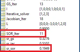
Minimum Spectral Radius for SOR Method
As we can see that the Spectral Radius is the minimum for the Successive Over -Relaxation Method(sr_sor). This Spectral Radius was achieved for a relaxation Factor, r= 0.9. A decrease or increase in the Relaxation factor was increasing the Spectral Radius thereby changing the Number of Iterations as well. Hence r=0.9 will be the ideal or Optimum Value of Relaxation Factor in this case.
6. A Diagonally dominant matrix is a square matrix such that in each row, the absolute value of the term on the diagonal is greater than or equal to the sum of absolute values of the rest of the terms in that row. So, if we remove the Diagonal Dominance of the matrix, the Spectral Radius increases in magnitude by a lot. Increase in Spectral Radius means that the Eigen values are higher which means that the convergence for that scheme is a lot tougher.
- Results:
1. We observed that how the Spectral Radius affects the convergence rates and how the diagonal dominance will also affect the Eigen Values and hence the Spectral Radius.
Here is the workspace for this code: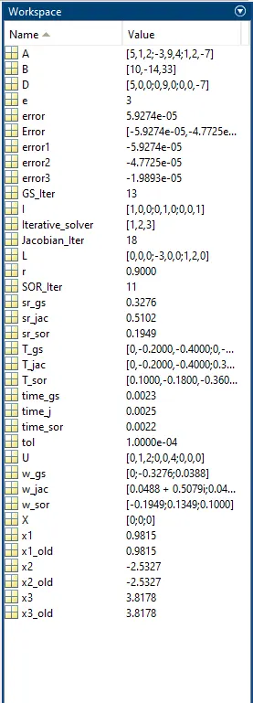
Workspace for the Code
As, we can see that the time taken for the jacobian method is larger than the other two methods, meaning that the time taken for convergence is higher in this method because the values are updated only after an entire iteration and not like in the Gauss-Sidel method, where the values from the left hand side are updated in between that iteration. This means that the Convergence is achieved faster in those methods.
2. We then plot the graphs between the Number of Iterations and the Magnification Factor for all the three Iterative Techniques.
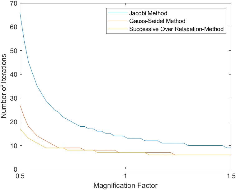
Here, we can see that, as the Magnification Factor increases from 0.5 to 1.5, the Number of Iterations decreases till magnification number=1 and then pretty much remains constant. This happens because as the Magnification number increases, the Diagonal Dominance of the matrix increases the stability of the matrix also increases and it tends towards convergence much faster.
3. The next we can plot is between Magnification factor and the Spectral Number. The plot is as follows: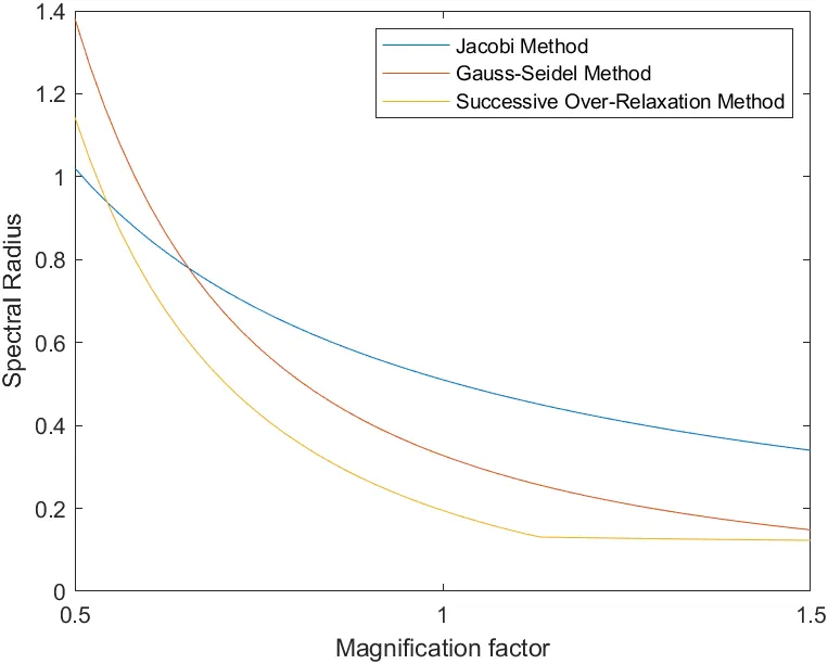
We can see that as the Magnification Factor increases from 0.5 to 1.5, the Spectral Radius is decreasing. As we have already seen that as the Magnification factor increases, the Number of Iterations decreases, and since the Number of Iterations is decreasing, we can conclude that the Convergence is becoming easier. Because the Convergence is becoming easier, the Spectral number will also go down as the Spectral Number represents the Maximum of the absolute values of the Eigen value of the Matrix, and we know that an eigenvector or characteristic vector of a linear transformation is a nonzero vector that changes by a scalar factor when that linear transformation is applied to it
4. The last graph that we need to plot is between Number of Iterations and the Spectral Radius. The plot is as follows: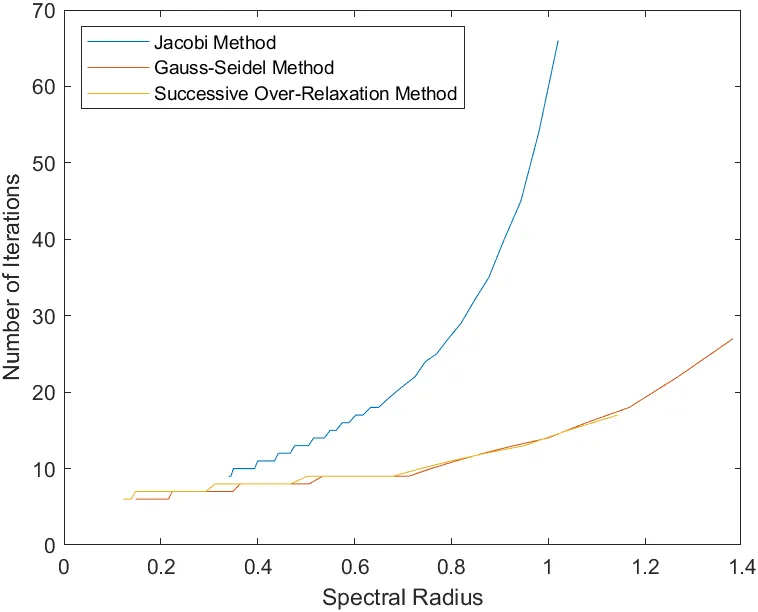
As we can see that as the Spectral Radius increases, the Number of Iterations also increases. The interesting point to note is that the slope for the Jacobi-Method is much larger than the other two methods. This increased slope tells us that for a minimal change in the Spectral Radius, the Number of Iterations increases by a large margin. It tells us that the relation between the Spectral Radius and the Number of Iterations is much more "sensitive" for the Jacobi-Method when we compare it with the other two methods. Even, when the Spectral Number is larger than 1, the solution diverges. This happens because, when we try to achieve a Spectral Radius greater than 1, the Solver has a tendency to over-jump the correct solution and it then tries to jump back and forth between the correct solution and the next calculated value. This happens till infinity and MATLAB does not produce a definite answer for it hence, no solution is calculated for it. - Conclusion: In conclusion, I would like to state that this challenge helped me understand the stability analysis for linear systems. Here, we understood the various parameters that will define the convergence rates for the three Iterative methods, namely, Jacobi Method, Gauss-Seidel Method and the Successive-Over Relaxation Method. We even understood the Diagonal Dominance of the Matrix and how it plays a role in the calculation of Spectral Radius of the Matrix.