Simulation of Quasi 1 D Supersonic nozzle flow simulation using MacCormack Method
AIM: Simulation of Quasi 1 D Supersonic nozzle flow simulation using MacCormack Method
OBJECTIVE:
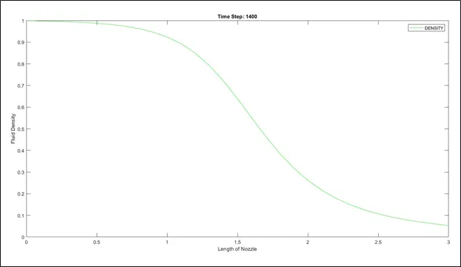
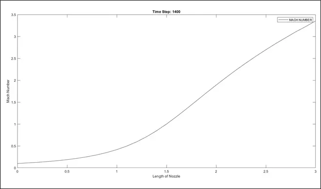
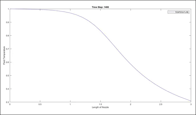
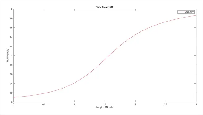
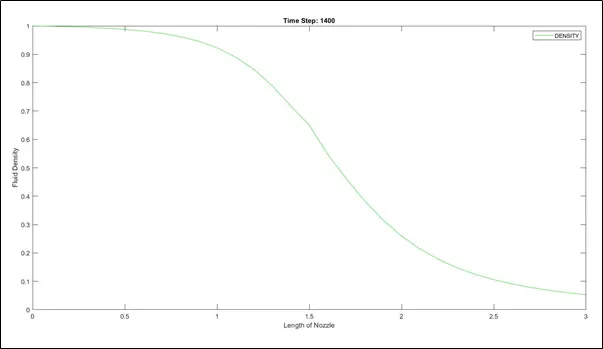
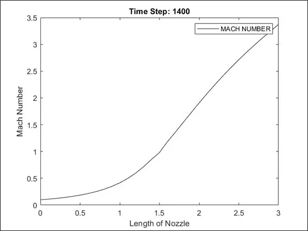
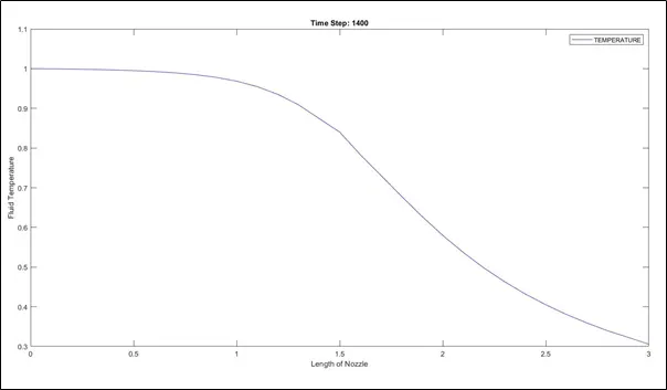
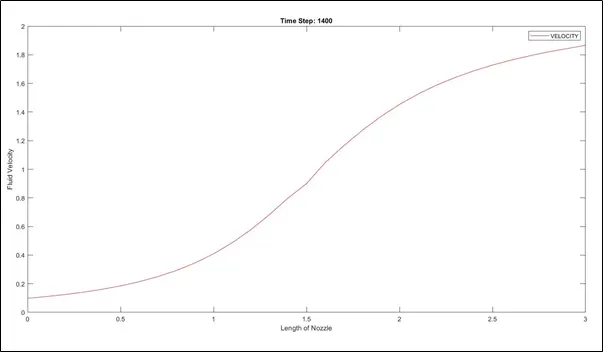
- Steady-state distribution of primitive variable inside the nozzle.
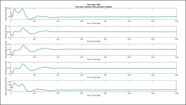
- Time-Wise variation of a primitive variable.
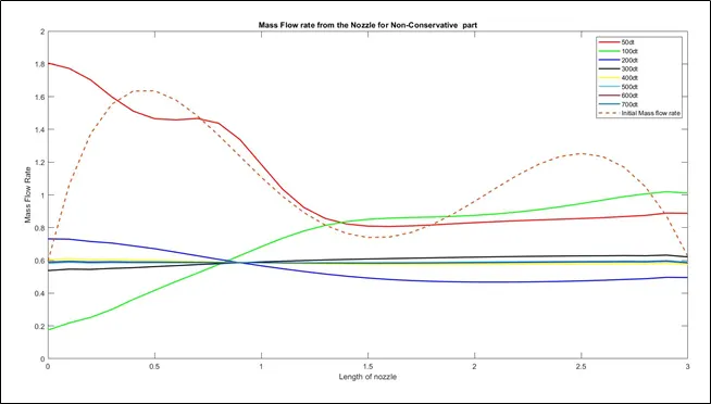
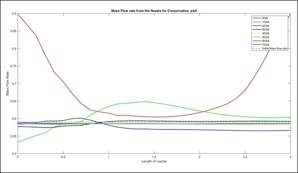
- Variation of mass flow rate distribution inside the nozzle at different time steps during the time marching process.
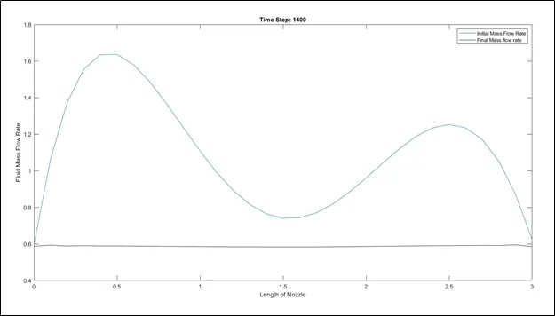
- Comparison of the normalized mass flow rate distribution of both forms.
INTRODUCTION OF PROBLEM/PHYSICAL ASPECT:
1D, steady, isentropic flow considered through the Convergent – Divergent nozzle. It is assumed that the nozzle is connected to the very large reservoir whose area is infinite. Hence, the velocity at the inlet is zero or negligible. Pressure and temperature at the inlet of the nozzle are P0 and T0.
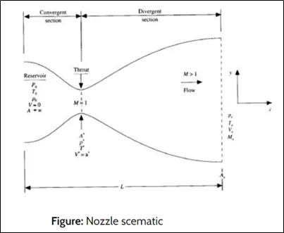
It is assumed that the flow properties are varying along the X – Direction only and at section flow properties are constant along the Y – Direction.
ANALYTICAL SOLUTION OF PROBEM:
Governing equations is as follows:
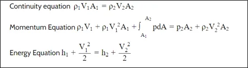
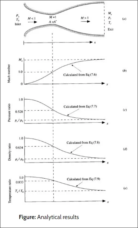
Solving the above equation analytically, we get the following results:
Solution by using CFD technique:
The solution is obtained using both conservative and non-conservative forms of governing equation.
Following are the governing equations in non-conservative form (Dimensional):
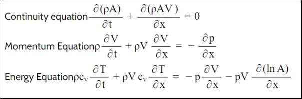
Following are the governing equations in non-conservative form (Non – Dimensional):
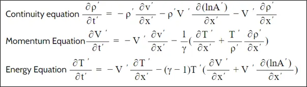
Where:

Please note that all prime quantities are non-Dimensional in nature.
Now, to solve the above equations using MacCormack Method (Predictor and Corrector method)
- Predictor step

- Corrector Step:
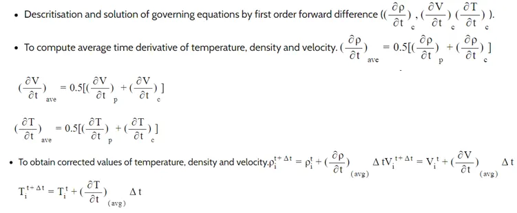
Calculation of Time Step:
Time step is calculated for all time steps using the following expression:
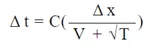
Where C = CFL number
Time step is calculated for all nodes and minimum of it is taken as time step for further calculation.
Nozzle Shape:
Nozzle shape is varying parabolically w.r.t.x as A = 1 + 2.2(x – 1.5)2 f OR 0 ≤ x ≤ 3
Initial Conditions:
The initial condition for density, velocity, and temperature is calculated from the following expression:

Boundary Conditions:
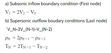
Solution using a non-conservative form of governing equation:
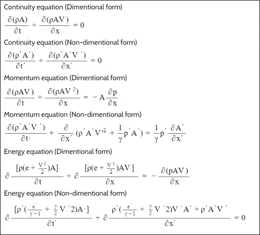
Now, let us define elements if solution vector U, the solution vector F, and the source term J as follows:
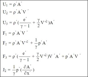
Substituting the above equations in governing differential equation, we get
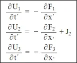
The above equations are governing differential equations for quasi 1D flow in conservative form.
Now from definitions U1, U2, and U3
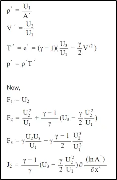
Initial Conditions:

Nozzle Shape:
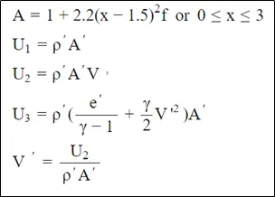
Boundary Conditions:
- Subsonic Inflow boundary condition (First Node):
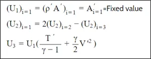
2. Supersonic outflow boundary condition (Last node):
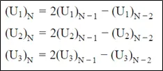
Main Code:
Non - Conservative Part:
clear all
close all
clc

%% Inputs
n = 31;
l = 3; % Length of domain
x = linspace(0,l,n);
dx = x(2)-x(1);
gamma = 1.4;

%% Initial Values

rho = 1-0.3146.*x;              % Density
T = 1-0.2314.*x;                % Temperature
V = (0.1+1.09.*x).*T.^0.5;      % Velocity

A = 1+2.2*(x-1.5).^2;           % Area

%% Time Step calculation by Courant no.
nt = 1400; % Total no. of time steps
%C = linspace(0.1,1,n); % Courant No. defined (0<=C<=1)
C = 0.5;
a = sqrt(T);
for i = 1:n
    dt_1 = C.*(dx./(a+V));
end

dt = min(abs(dt_1));

%% Therotical mass flow rate
for i = 1:n
    m_initial(i) = rho(i)*A(i)*V(i);
end

%% Outer time loop (Solving using McCormack Method)

for j = 1:nt

    % Saving the old values
        rho_old = rho;
        V_old = V;
        T_old = T;

    % Predictor method
    for k = 2:(n-1)

        % Splitting the values of easyfication

        dvdx = (V(k+1)-V(k))/dx;
        drhodx = (rho(k+1)-rho(k))/dx;
        dlogadx = (log(A(k+1))-log(A(k)))/dx;
        dTdx = (T(k+1)-T(k))/dx;

        % Continuity Equation
        drho_dt_p(k) = -rho(k)*(dvdx)-rho(k)*V(k)*(dlogadx)-V(k)*(drhodx);

        % Momentum Equation
        dv_dt_p(k) = -V(k)*(dvdx)-(1/gamma)*(dTdx + (T(k)/rho(k))*drhodx);

        % Energy Equation
        dT_dt_p(k) = -V(k)*(dTdx)-(gamma-1)*T(k)*(dvdx + V(k)*dlogadx);


        % Solution Update
        rho(k) = rho(k) + drho_dt_p(k)*dt;
        V(k) = V(k) + dv_dt_p(k)*dt;
        T(k) = T(k) + dT_dt_p(k)*dt;

    end


    % Corrector method
    for k = 2:(n-1)

        % Splitting the values of easyfication

        dvdx = (V(k)-V(k-1))/dx;
        drhodx = (rho(k)-rho(k-1))/dx;
        dlogadx = (log(A(k))-log(A(k-1)))/dx;
        dTdx = (T(k)-T(k-1))/dx;

        % Continuity Equation
        drho_dt_c(k) = -rho(k)*(dvdx)-rho(k)*V(k)*(dlogadx)-V(k)*(drhodx);

        % Momentum Equation
        dv_dt_c(k) = -V(k)*(dvdx)-(1/gamma)*(dTdx + (T(k)/rho(k))*drhodx);

        % Energy Equation
        dT_dt_c(k) = -V(k)*(dTdx)-((gamma-1)*T(k))*(dvdx + V(k)*dlogadx);

    end

    % Compute the average time derivative

    dvdt = 0.5*(dv_dt_p + dv_dt_c);
    drhodt = 0.5*(drho_dt_p + drho_dt_c);
    dTdt = 0.5*(dT_dt_p + dT_dt_c);

    % Final Solution Update
    for k = 2:n-1
        rho(k) = rho_old(k) + drhodt(k)*dt;
        V(k) = V_old(k) + dvdt(k)*dt;
        T(k) = T_old(k) + dTdt(k)*dt;
    end

    % Defining the Boundary Conditions
    % Inlet
    V(1) = 2*V(2)-V(3);
    rho(1) = 1;
    T(1) = 1;

    %Outlet
    V(n) = 2*V(n-1) - V(n-2);
    rho(n) = 2*rho(n-1) - rho(n-2);
    T(n) = 2*T(n-1) - T(n-2);

    % Calculating the Mach No. and pressure
    a = sqrt(T);
    M = V./a;
    p = rho.*T;

    % Calculating the mass flow rate along the length of the nozzle
    m = rho.*A.*V;

    % Calculation of primitive variables at throat
    rho_t(j) = rho(16);
    V_t(j) = V(16);
    T_t(j) = T(16);
    p_t(j) = p(16);
    M_t(j) = M(16);
    m_t(j) = m(16);

    % Plotting

    figure(6)
    if j==50
        plot(x,m,'r','linewidth',1.5)
        hold on
    else if j==100
        plot(x,m,'g','linewidth',1.5)
        hold on
        else if j==200
            plot(x,m,'b','linewidth',1.5)
            hold on
            else if j==300
                plot(x,m,'black','linewidth',1.5)
                hold on
                else if j==400
                    plot(x,m,'y','linewidth',1.5)
                    hold on
                    else if j==500
                        plot(x,m,'linewidth',1.5)
                        hold on
                        else if j==600
                            plot(x,m,'linewidth',1.5)
                            hold on
                            else if j==700
                                plot(x,m,'linewidth',1.5)
                                hold on

                                plot(x,m_initial,'--','linewidth',1.5)

                                xlabel('Length of nozzle');
                                ylabel('Mass Flow Rate');
                                legend('50dt','100dt','200dt','300dt','400dt','500dt','600dt','700dt','Initial Mass flow rate')
                                title('Mass Flow rate from the Nozzle for Non-Conservative  part')
                                end
                            end
                        end
                    end
                end
            end
        end
    end
end

figure(1)
plot(x,V,'r')
xlabel('Length of Nozzle');
ylabel('Fluid Velocity');
legend('VELOCITY');
title(sprintf('Time Step: %d',j));

figure(2)
plot(x,rho,'g')
xlabel('Length of Nozzle');
ylabel('Fluid Density');
legend('DENSITY');
title(sprintf('Time Step: %d',j));

figure(3)
plot(x,T,'b')
xlabel('Length of Nozzle');
ylabel('Fluid Temperature');
legend('TEMPERATURE');
title(sprintf('Time Step: %d',j));

figure(4)
plot(x,M,'black')
xlabel('Length of Nozzle');
ylabel('Mach Number');
legend('MACH NUMBER');
title(sprintf('Time Step: %d',j));

figure(5)
plot(x,m_initial)
hold on
plot(x,m,'black')
xlabel('Length of Nozzle');
ylabel('Fluid Mass Flow Rate');
legend('Initial Mass Flow Rate','Final Mass flow rate');
title(sprintf('Time Step: %d',j));

pause(0.01)
hold off

figure(7)
subplot(511)
plot(1:j,V_t,'linewidth',1.5)
xlabel('No. of Time Step')
ylabel('Velocity at Throat')
txt1 = (sprintf('Time Step: %d',j));
txt2 = ('Time-wise variation of the primitive variables');
title({txt1,txt2})

subplot(512)
plot(1:j,rho_t,'linewidth',1.5)
xlabel('No. of Time Step')
ylabel('Density at Throat')

subplot(513)
plot(1:j,T_t,'linewidth',1.5)
xlabel('No. of Time Step')
ylabel('Temperature at Throat')

subplot(514)
plot(1:j,p_t,'linewidth',1.5)
xlabel('No. of Time Step')
ylabel('Pressure at Throat')

subplot(515)
plot(1:j,M_t,'linewidth',1.5)
xlabel('No. of Time Step')
ylabel('Mach Number at Throat')
Conservative Part:
clear all
close all
clc

%% Inputs (Defining the mesh size)
n = 31;
l = 3; % Length of domain
x = linspace(0,l,n);
dx = x(2)-x(1);
gamma = 1.4;

%% Initial Values

A = 1+2.2*(x-1.5).^2;           % Area of nozzle

% Primitive variable of the nozzle

% The primitive variable Temperature and Density were kept constant and the
% third primitive variable Velocity was kept floating with the grid point

for i = 1:n

    if (x(i)>=0 && x(i)<=0.5)
        rho(i) = 1;
        T(i) = 1;

    elseif (x(i)>0.5 && x(i)<=1.5)
        rho(i) = 1-0.366*(x(i)-0.5);
        T(i) = 1-0.167*(x(i)-0.5);

    elseif (x(i)>1.5 && x(i)<=3)
        rho(i) = 0.634-0.3879*(x(i)-1.5);
        T(i) = 0.833-0.3507*(x(i)-1.5);
    end

    % For finding the floating variable of velocity, we use the mass flux
    % variable U2 which is nothing but 'm_dot'. Where m_dot is nothing but
    % the initial value of mass flow rate.

    % m_initial(i) = rho(i)*A(i)*V(i)
    % V(i) = m_initial(i)/(rho(i)*A(i))

    m_initial(i) = 0.59; % Therotical value of mass flow rate

    V(i) = m_initial(i)/(rho(i).*A(i));

end

%% Speed of sound and time step
a = sqrt(T);
nt = 1400;          % Total no. of time steps

%% Derived flux variable of the nozzle

U1 = rho.*A;
U2 = rho.*A.*V;
U3 = rho.*A.*((T/(gamma-1))+(gamma/2)*V.^2);

%% Outer time Loop (Solving using McCormack Method)

for j = 1:nt

    % The governing equation of Continuity, Momentum, and Energy has been
    % expressed in terms of flux variables

    % Continuity Equation   =   dU1/dt+dF1/dx=0
    % Momentum Equation     =   dU2/dt+dF2/dx=J2
    % Energy Equation       =   dU3/dt+dF3/dx=0

    % Saving the old values
        U1_old = U1;
        U2_old = U2;
        U3_old = U3;

        F1 = U2;
        F2 = (U2.^2./U1)+(((gamma-1)/gamma)*(U3-((gamma*0.5*(U2.^2))./U1)));
        F3 = ((gamma*U2.*U3)./U1)-((gamma*0.5*(gamma-1)*(U2.^3))./(U1.^2));

        %% Time Step calculation by Courant no.
        %nt = 1400; % Total no. of time steps
        C = 0.5;
        %for i = 1:n
            dt_1 = C*(dx./(a+V));
        %end

        dt = min(abs(dt_1));


        % Predictor Method
        for k = 2:(n-1)

            J2(k) = (1/gamma)*rho(k)*T(k)*((A(k+1)-A(k))/dx);

            % Continuity Equation
            dU1_dt_p(k) = -(F1(k+1)-F1(k))/dx;

            % Momentum Equation
            dU2_dt_p(k) = -(F2(k+1)-F2(k))/dx+J2(k);

            % Energy Equation
            dU3_dt_p(k) = -(F3(k+1)-F3(k))/dx;


            % Solution Update
            U1(k) = U1(k) + dU1_dt_p(k)*dt;
            U2(k) = U2(k) + dU2_dt_p(k)*dt;
            U3(k) = U3(k) + dU3_dt_p(k)*dt;

            rho(k) = U1(k)/A(k);
            V(k) = U2(k)/U1(k);
            T(k) = (gamma-1)*((U3(k)/U1(k)) - ((gamma/2)*(V(k)^2)));
        end

        F1 = U2;
        F2 = (U2.^2./U1)+(((gamma-1)/gamma)*(U3-((gamma*0.5*(U2.^2))./U1)));
        F3 = ((gamma*U2.*U3)./U1)-((gamma*0.5*(gamma-1)*(U2.^3))./(U1.^2));


        % Corrector Method

        for k = 2:(n-1)

            J2(k) = (1/gamma)*rho(k)*T(k)*((A(k)-A(k-1))/dx);

            % Continuity Equation
            dU1_dt_c(k) = -(F1(k)-F1(k-1))/dx;

            % Momentum Equation
            dU2_dt_c(k) = -(F2(k)-F2(k-1))/dx+J2(k);

            % Energy Equation
            dU3_dt_c(k) = -(F3(k)-F3(k-1))/dx;
        end

        % Computing the average time derivative

        dU1_dt = 0.5*(dU1_dt_p+dU1_dt_c);
        dU2_dt = 0.5*(dU2_dt_p+dU2_dt_c);
        dU3_dt = 0.5*(dU3_dt_p+dU3_dt_c);

        % Performing the final solution update

        for i = 2:(n-1)
            U1(i) = U1_old(i) + dU1_dt(i)*dt;
            U2(i) = U2_old(i) + dU2_dt(i)*dt;
            U3(i) = U3_old(i) + dU3_dt(i)*dt;
        end

        % Defining the boundary conditions
        % Inlet
        U1(1) = rho(1)*A(1);
        U2(1) = 2*U2(2)-U2(3);
        U3(1) = U1(1)*((T(1)/(gamma-1))+(0.5*gamma*(V(1)^2)));

        %Outlet
        U1(n) = 2*U1(n-1)-U1(n-2);
        U2(n) = 2*U2(n-1)-U2(n-2);
        U3(n) = 2*U3(n-1)-U3(n-2);

        % Density Update
        rho = U1./A;

        % Velocity Update
        V = U2./U1;

        % Temperature Update
        T = (gamma-1)*((U3./U1) - ((gamma/2)*(V.^2)));

        % Calculating the Mach No.
        a = sqrt(T);
        M = V./a;
        p = rho.*T;

        % Calculating the mass flow rate along the length of the nozzle
        m = rho.*A.*V;

        % Calculation of primitive variables at throat
        rho_t(j) = rho(16);
        V_t(j) = V(16);
        T_t(j) = T(16);
        p_t(j) = p(16);
        M_t(j) = M(16);
        m_t(j) = m(16);

        % Plotting

    figure(6)
    if j==50
        plot(x,m,'r','linewidth',1.5)
        hold on
    else if j==100
            plot(x,m,'g','linewidth',1.5)
            hold on
        else if j==200
                plot(x,m,'b','linewidth',1.5)
                hold on
            else if j==300
                    plot(x,m,'black','linewidth',1.5)
                    hold on
                else if j==400
                        plot(x,m,'y','linewidth',1.5)
                        hold on
                    else if j==500
                            plot(x,m,'linewidth',1.5)
                            hold on
                        else if j==600
                                plot(x,m,'linewidth',1.5)
                                hold on
                            else if j==700
                                    plot(x,m,'linewidth',1.5)
                                    hold on

                                    plot(x,m_initial,'--','linewidth',1.5)

                                xlabel('Length of nozzle');
                                ylabel('Mass Flow Rate');
                                legend('50dt','100dt','200dt','300dt','400dt','500dt','600dt','700dt','Initial Mass flow rate')
                                title('Mass Flow rate from the Nozzle for Conservative  part')
                                end
                            end
                        end
                    end
                end
            end
        end
    end
end

figure(1)
plot(x,V,'r')
xlabel('Length of Nozzle');
ylabel('Fluid Velocity');
legend('VELOCITY');
title(sprintf('Time Step: %d',j));

figure(2)
plot(x,rho,'g')
xlabel('Length of Nozzle');
ylabel('Fluid Density');
legend('DENSITY');
title(sprintf('Time Step: %d',j));

figure(3)
plot(x,T,'b')
xlabel('Length of Nozzle');
ylabel('Fluid Temperature');
legend('TEMPERATURE');
title(sprintf('Time Step: %d',j));

figure(4)
plot(x,M,'black')
xlabel('Length of Nozzle');
ylabel('Mach Number');
legend('MACH NUMBER');
title(sprintf('Time Step: %d',j));

figure(5)
plot(x,m_initial,'linewidth',1.5)
hold on
plot(x,m,'black','linewidth',1.5)
xlabel('Length of Nozzle');
ylabel('Fluid Mass Flow Rate');
axis([0 1 0 1]);
legend('Initial Mass Flow Rate','Final Mass flow rate');
title(sprintf('Time Step: %d',j));

pause(0.01)
hold off

figure(7)
subplot(511)
plot(1:j,V_t,'linewidth',1.5)
xlabel('No. of Time Step')
ylabel('Velocity at Throat')
txt1 = (sprintf('Time Step: %d',j));
txt2 = ('Time-wise variation of the primitive variables');
title({txt1,txt2})

subplot(512)
plot(1:j,rho_t,'linewidth',1.5)
xlabel('No. of Time Step')
ylabel('Density at Throat')

subplot(513)
plot(1:j,T_t,'linewidth',1.5)
xlabel('No. of Time Step')
ylabel('Temperature at Throat')

subplot(514)
plot(1:j,p_t,'linewidth',1.5)
xlabel('No. of Time Step')
ylabel('Pressure at Throat')

subplot(515)
plot(1:j,M_t,'linewidth',1.5)
xlabel('No. of Time Step')
ylabel('Mach Number at Throat')
Results:
Non-Conservative form of Governing Equations at n = 31:
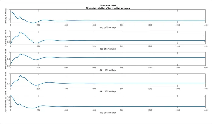
Mass flow rate from the nozzle for the non-conservative part at various time steps:
Comparisons of initial and Final mass flow rate:
DENSITY:
MACH NUMBER:
TEMPERATURE:
VELOCITY:
Conservative form of Governing Equations at n = 31:
Mass flow rate from the nozzle for the conservative part at various time steps:
DENSITY:
MACH NUMBER:
TEMPERATURE:
VELOCITY:
Discussion and Conclussion:
- Mass flow distribution in conservative form is much closer to the analytical value and it is somewhat constant. But in the case of non - conservative form, there is a sizeable variation in mass flow distribution.
- The non - conservative form leads to a smaller residual. Hence, in terms of the quality of the algorithm, non - conservative form does a better job.
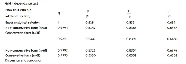
- Both the form of governing differential equations are satisfactory if we compare them with analytical form.
- It almost takes 600 iterations to have a steady-state solution.
- The solution is grid-independent.