Shock tube simulation project
AIM: To set up a shock tube with a high-pressure differential between the two regions (low and high-pressure region filled with O2 and N2 gas respectively) and simulate the formation of shocks as a result of rupture of the diaphragm that separates these two regions from each other
THEORY
The shock tube is an instrument used to replicate and direct blast waves at a sensor or a model in order to simulate actual explosions and their effects, usually on a smaller scale. Shock tubes (and related impulse facilities such as shock tunnels, expansion tubes, and expansion tunnels) can also be used to study aerodynamic flow under a wide range of temperatures and pressures that are difficult to obtain in other types of testing facilities. Shock tubes are also used to investigate compressible flow phenomena and gas phase combustion reactions. More recently, shock tubes have been used in biomedical research to study how biological specimens are affected by blast waves.
GEOMETRY
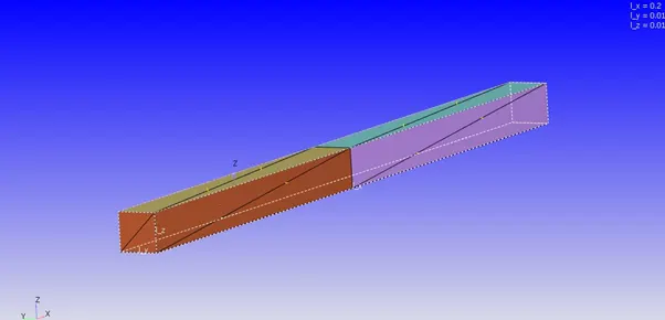
The length of the entire shock tube (x-direction) is 0.2m, the length of the high-pressure and low-pressure region is 0.1m. The width and height of the tube are 0.01m.
CASE SETUP
Application Type: Time based
Species: N2,O2
1.Simulation Parameters
1.1 Run parameters: Solver= Transient-state solver
Simulation mode= Full hydrodynamic
Gas flow solver= Compressible
1.2 Simulation Time Parameters: Start time= 0.0s
End time= 0.003s
Initial time-step= 1e-7s
Minimum time-step= 1e-7
Maximum time-step= 1e-5
1.3 Solver parameters:
Navier-Stokes solver scheme= PISO
Navier-Stokes solver type= density-based
2.Boundary Conditions
Two boundaries defined
- a) High-pressure boundary (Region assigned= High-pressure region)
- b) Low-pressure boundary (Region assigned= Low-pressure region)
Both the boundaries are provided with the stationary wall, slip boundary condition
3.Regions and Initialization
- a) High-pressure region
Species= N2
Pressure= 600000 Pa
2.a) Low-pressure region
Species= O2
Pressure= 101325 Pa
3.1 Events
Events described below are between regions
- a) Event= Close (0-0.001s)
- b) Event= Open (0.001-0.003s)
Physical model
4.1 Turbulence model:RNG K-epsilon turbulence mode
5.Grid Control
5.1 Base grid: 0.002m in all three coordinate axes.
5.2 Adaptive mesh refinement:
Active regions= high-pressure region, low-pressure region
AMR by species N2
Timing type= Permanent
SGS embed= 0.001
Start and end time= 0-0.003s
Embed scale= 3
RESULT
MESH GENERATION
PLOT 1:Cell count
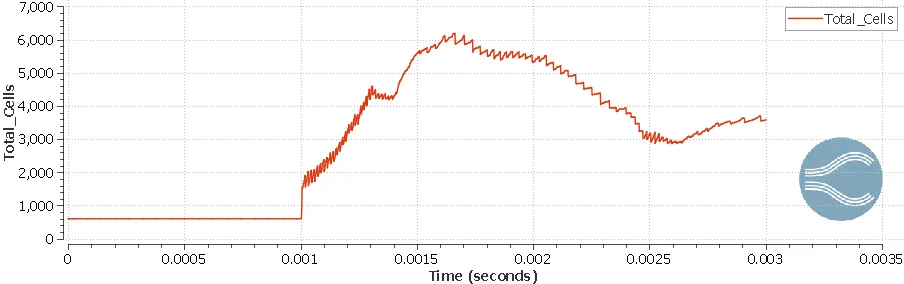
The diaphragm between high pressure region and low pressure region opens up after 0.001 seconds, i.e. why the number of cells starts increasing due to Adaptive mesh refining after this time step.
PRESSURE CONTOUR
Plot 2:Pressure variation plot
Plot 3:Miniimum pressure in the entire region
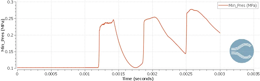
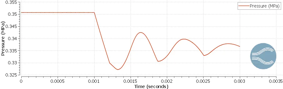
from the figure given above the minimum pressure is plotted in the domain. the minium pressure is in the oxygen region which is at 1 bar but as soon as the diaphragm opens up the minimum pressure increases to certain level as the solution progresses.
Plot 4:Maximum pressure in the entire region
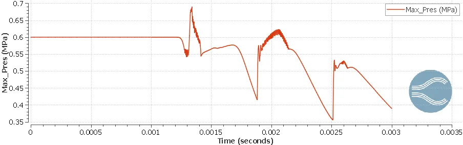
As you can see in the figure given above that the maximum pressure in the region is 6 bar. and as soon as the diaphragm opens up the maimum pressure drop in the region and as the simulation progresses towards equilibrium the max pressure value decreases.
TEMPERATURE CONTOUR
Plot 5:Mean Temperature in the region
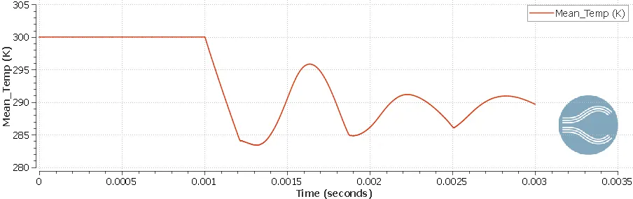
Above figure shows the mean temperature variation during shock Flow as the flow between the region takes place, temperature starts fluctuating but at the end of the cycle the mean tmeperature is nearly the same.
Plot 6:Minimum temperature in the region
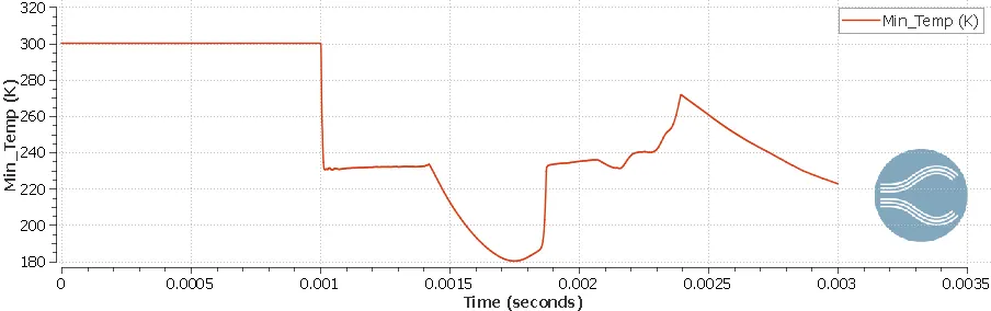
the minimum temperature in the domain also changes as the pressure changes during the flow inside the domain so is the temperature its minimum value goes upto 180 K, where as at the end of the cycle its value reaches 230 K.
Plot 7:Maximum Temperature in the region
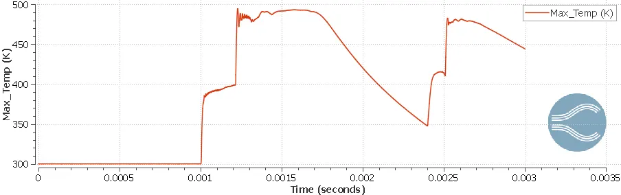
the initial temperature inside both the region is taken as 300 K but as soon as the flow takes place the temperature started fluctuating and at the end of the cycle its value reaches upto 470 K.