Roof Crush Impact Simulation on a Dodge Neon BIW Model with FMVSS 216 Impactor using Hypermesh and RADIOSS.
Project-3 Report.
- Aim: To perform the deck set up and run the Roof Crush Impact Simulation on the given Dodge Neon BIW Model with a Federal Motor Vehicle Safety Standard (FMVSS) 216 Impactor.
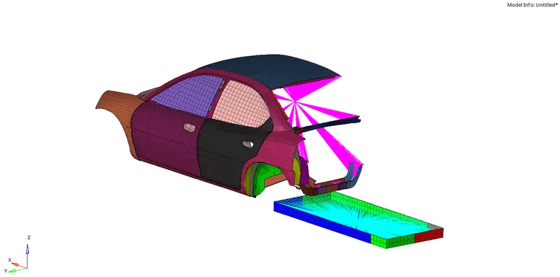
Initial model - Objective: 1. To place the Impactor at the appropriate loaction right above the roof.
2. To create Appropriate Contact Interface wherever needed.
3. To change the Boundary conditions on the Suspension Tower and the Impactor.
4. To give an Initial Displcement to the Impactor.
5. To request certain Animation files in the Time history of the simulation. - Procedure:
1. The very first step in the solver deck setup of this model is to check the units in which the Geometry has been modelled. To do this, we need to use the Begin card in the Model tab as shown. Here we can view the basic units of Mass, Length and time that were used in the model.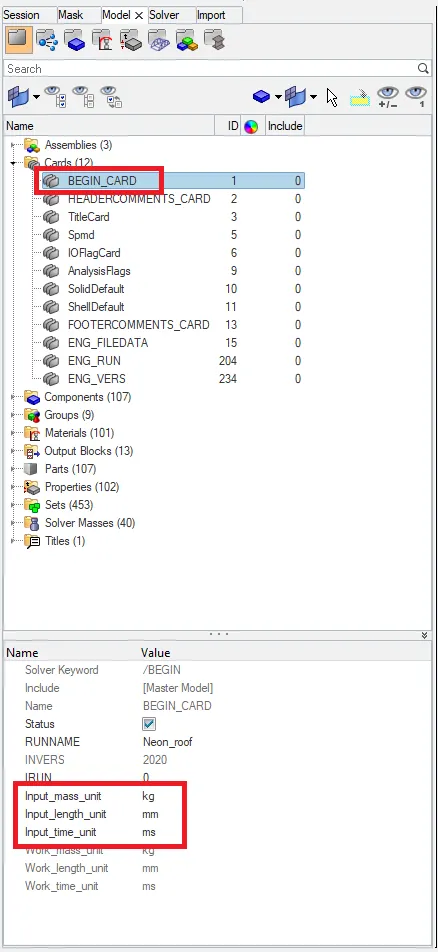
Begin Card
We can see that the units of Mass, Length and Time are Kg,mm and ms respectively.
2. The next step is to position the Impactor at the exact location so that the Roof Crush simulation can take place appropriately. To do this, we simply need to use the rotate and translate command in the Tool Tab.
1D -> Translate and rotate command
Translate command
Rotate command
We simply need to follow the steps in the order given below to position the Impactor at the right location:
1. A 180° rotation about the global z-axis with the point opposite to C as base point
2. A -5° rotation about the axis through axis AB
3. A 25° rotation about the axis through axis AC
4. A translation to put point A at global ( -3500.00, 584.822, 1343.06)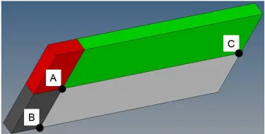
FMVSS 216 Impactor
After following these commands properly, we will get the impactor at the desired location as shown below: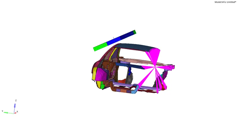
Final Positioning of the Impactor
3. After the positioning of the impactor is done, we then go onto creating the Type7 contact interface between the impactor and the car. We must also create another Type7 contact interface for the self impact of the vehicle. To create a Type7 contact, we must right click on the Tree and use the create option. Under this, we must select the Contact interface command as shown below: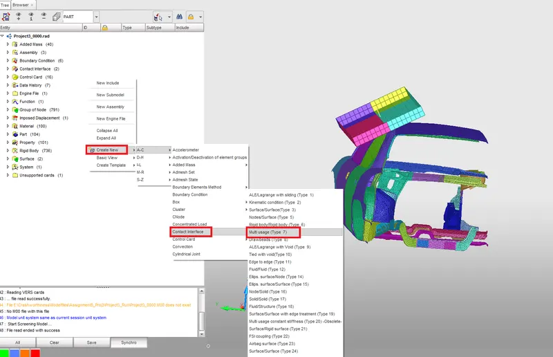
Create -> Type7 Contact
Like this, we can create a Type 7 contact. Now in this contact we need to define the basic properties such as Igap, Istiff, Inacti etc. We simply change their value to the recommended values.
Here are the recommended values for a Type7 Contact:
1. Istf = 4 (Stiffness based on Softer segment.)
2. Igap = 2 (Variable Gap taken into account.)
3. Idel = 2 (Remove Slave nodes from contact because of element deletion.)
4. Inacti = 6 (Reduce gap by 30% more than the defined gap.)
5. Iform = 2 (Frictional forces are calculated according to the Stiffness parameters.)
6. Stmin = 1KN/mm (Minimum stiffness to avoid a too soft contact.)
When defining the Contact between the Impactor and the car, the master segment will be the Impactor and the slave segment will be the Car model. This is because there is a much coarse mesh on the Impactor making the impactor much stiffer than the Car in this case. Also, the body under study is the car model and we want results and simulations for it, hence it is to be kept as the slave segment.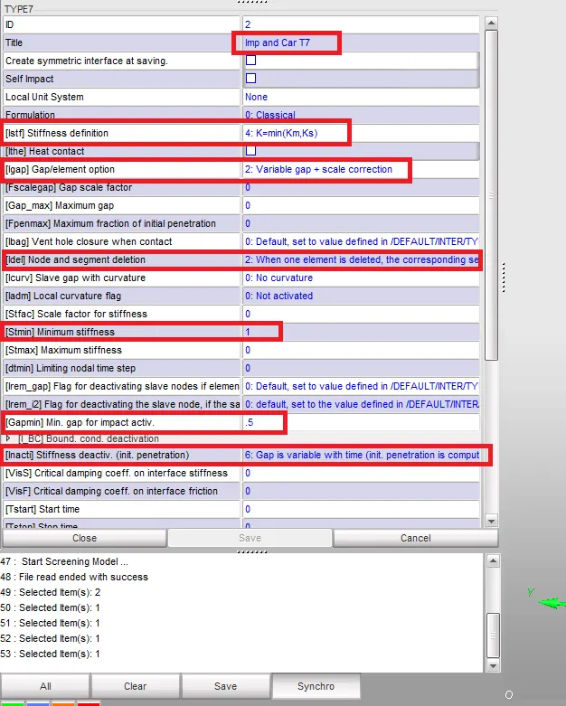
Type7 contact between Impactor and Car
When defining the Self impact contact, we will give the car model as both the slave and the master segment as we want to prevent the Car model from collapsing in itself. Since we have defined the slave and master as the car, the algorithm does not allow the master segment (car model) to penetrate the slave segment (car model), hence the self collapsing will not occur.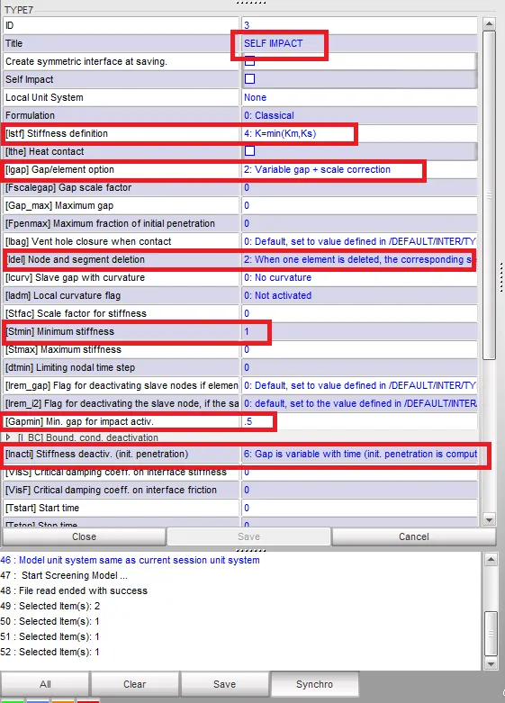
Type7 Self Impact Contact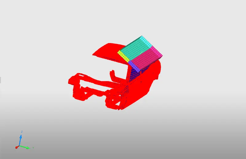
Self Impact Contact Defined
We will give the value of friction as 0.2 as mentioned in the question. Also, we will give the value of Iform here: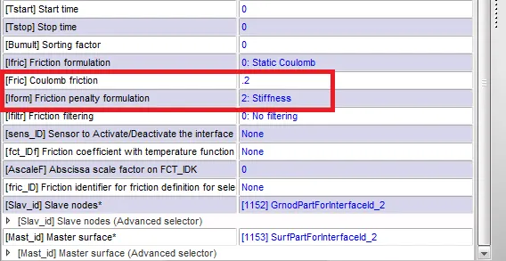
Friction value given
4. After this step, we need to check all the rigid body connections in the model. To see if we have appropriate connections defined throughout the model, we need to do it by visual inspection. So, for this, we simply move around the model and check if two surfaces are connected appropriately. Any two surfaces that have a gap between them must be connected using either Rigid Body connections or even springs in some cases.
In case we get two surfaces, where the contact is not appropriately defined, we then need to add a Rigid body Element or maybe a Spring Element.
In our case, a lot of the components were not connected by rigid bodies. Like, for example, these two components were not connected by a Rigid Body: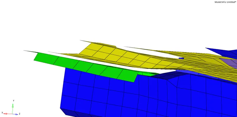
Before making the Rigid Body connections
To add rigids, we can use the Rigid command under the 1D tab as shown below:
1D -> Rigids

Rigids command
After we select two or more nodes, those two components will be connected by a RBE2 (Rigid Body Element) that will hold those components in place. An RBE2 element has inifinite stiffness, it will not deform under excessive loads.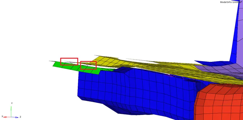
After giving the Rigid Body connection
5. The next step is to change the boundary conditions of certain nodes in the certain components. To create a Boundary condition, we must first create it. To create the Boundary condition, we must right click on the tree and use the create option. In create, we need to use the Boundary Conditions command as shown: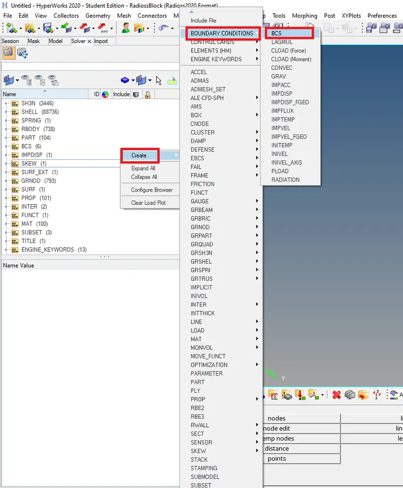
Create -> Boundary Condition
After creating a Boundary condition, we must alter the Degree of Freedom on the node/nodes selected. There are 6 Degrees of Freedom as we know, i.e. 3 in Translation and 3 in Rotation. For example, when we create a new boundary condition, we get to select all the Different DOF's we want locked and which ones we want free.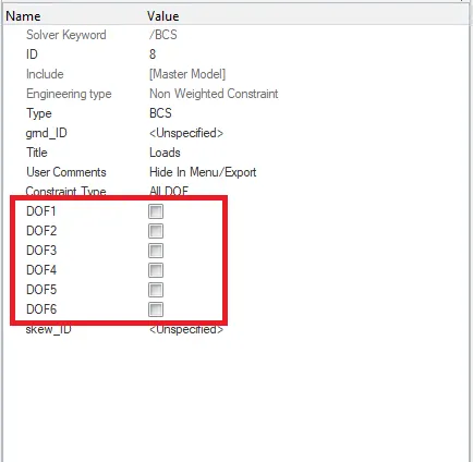
Degree of Freedom in the BCS
DOF's 1,2,3 are Translation in x,y,z resepctively and the DOF's 4,5,6 are Rotation in x,y,z.
So, When we check any DOF from the above box, we basically lock or restrict the motion of the body in that direction. So, for example, if we check DOF3, then the body will not be able to translate in the global z axis or, if we check DOF 5, then the rotation of the body will be restricted in the global y axis.
So, when we had to keep the suspension shock tower nodes locked in Z direction, we simply checked the DOF3 and let all the other different motions occur.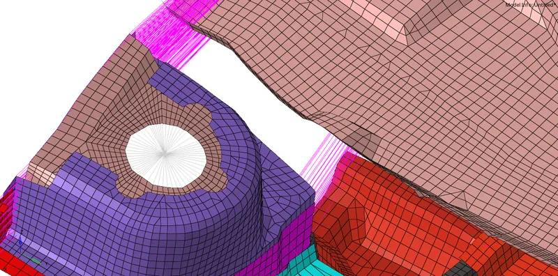
Before giving the Boundary condition
We then edit the DOF's as per requirement.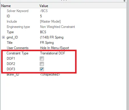
DOF constraints
Now we get the final Boundary Condition applied: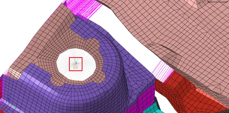
After giving the Boundary condition
Just like this we must give a Boundary Condition to both the ends of the Impactor Springs as well.
But when are putting the BCS for the impactor spring, we must create a Skew to put it as a directional support to the lower end of the spring so that it moves in a particular direction.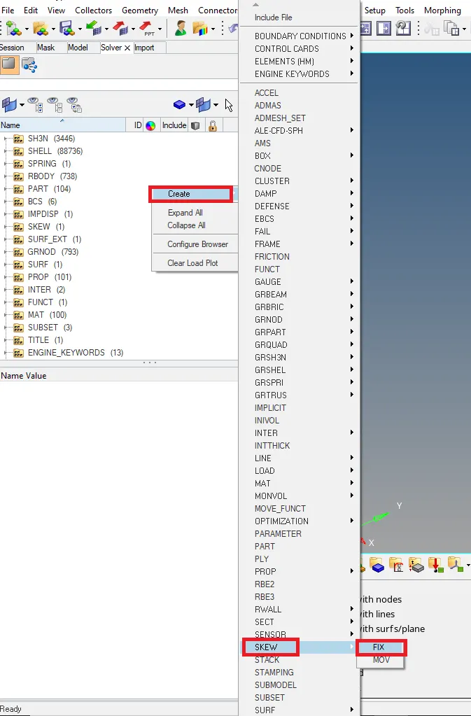
Create -> SKEW
Like this we can create a skew and give it the three nodes so to define the three axes of it. We need to define such that the Z-axis of the skew must be towards the car.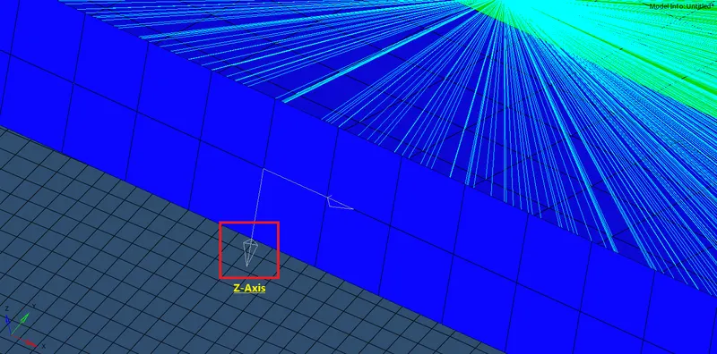
Skew created
Now, we can add this skew to the BCS where we have to the lower node of the Impactor spring.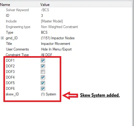
Skew system added
As we can see, only the movement in the Z-axis of the Skew system is added. Similarly, we can go on to create all the Skew Systems for the model.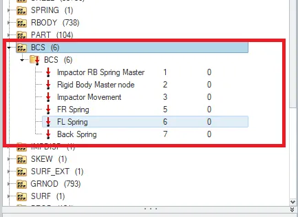
All the Boundary Conditions applied on the model
6. The next step is to give an Imposed Displacement on the impactor so that it goes and hits the roof of the vehicle. To give an Imposed Displacement, we must put in a curve in the form of a graph as input. To create an Imposed Displacement in the form of a boundary condition, we simply need to create a Boundary condition. So, to do this, we need to right click on the tree and use the option of Create. In this option, we just need to use the command of Boundary conditions and create and Imposed displacement.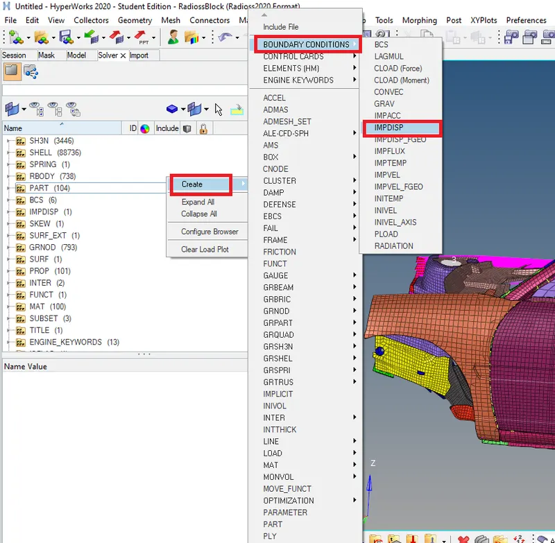
Create -> Imposed Displacement
Like this, we can add an Imposed Displacement to the needed nodes. Then, we need to give in the necessary inputs for it.
The grnd_ID is all the nodes where we want the Imposed displacement to be applied. In ourr case, we can simply give the Imposed displacement to be at the Master node of the Rigid body connecting all the nodes of the impactor. If the Master node is moving towards the direction of the vehicle, it will bring all the nodes that it is connecting, i.e. the entire Impactor with it.
The fct_ID(T) is the function where we describe the Displacement with respect to time. So, here, we give the input such that we plot a the Displacement vs Time graph. We know that at T(time) = 0ms, the D(Displacement) = 0mm and at T = 200ms the D = 200mm, using this Data, we need to plot the graph and give this graph as an input at this location.
The Skew_ID is the input for the Skew system that needs to be given.
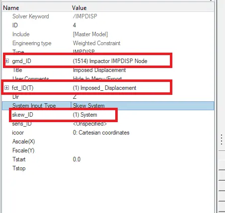
Imposed Displacement Properties
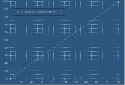
Imposed Displacement Curve
7. The next step is to set the Time-Steps for the simulation. To do this, we simply need t oadd the necessary cards and then change the values of it.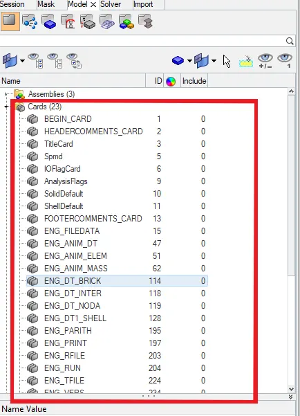
All the Defined Cards
If any card is missing, we can then add those certain cards by using the option of Control cards under the Analysis tab as shown below:
Analysis -> Control Cards
Since, all the cards have been added, the following cards are needed to change the Time-Steps of the Simulation:
a. ENG_DT_BRICK : Tscale: 0.67 ; Tmin: 0.0001
b. ENG_DT_INTER : Tscale: 0.67 ; Tmin: 0.0005
c. ENG_DT_NODA : Tscale: 0.67 ; Tmin: 0.0005
d. ENG_DT1_SHELL : Tscale: 0.67 ; Tmin: 0.0
All the other cards have their own reasons/meanings to be added, like for example:
a. ENG_RUN: 200.0 ms (run time for the simulation)
b. ENG_TFILE: Tfreq = 0.1. (frequency at which the Time History is plotted)
c. ENG_ANIM_DT: Tfreq = 5.0 (frequency at which the Animation files will be written)
d. ENG_ANIM_ELEM: Here we need to check all the Elemental Animation output requests from the solver.
e. ENG_PARITH: Turns the parallel Arithmetic ON/OFF
f. ENG_RFILE: Writes the restart File.
g. ANALY card: Defines the type of analysis and sets analysis flags.
8. The last step before running the simulation is to request for the Time-History of the simulation. To do this, we need to create a Time history and then select the Type of Time-History that we need.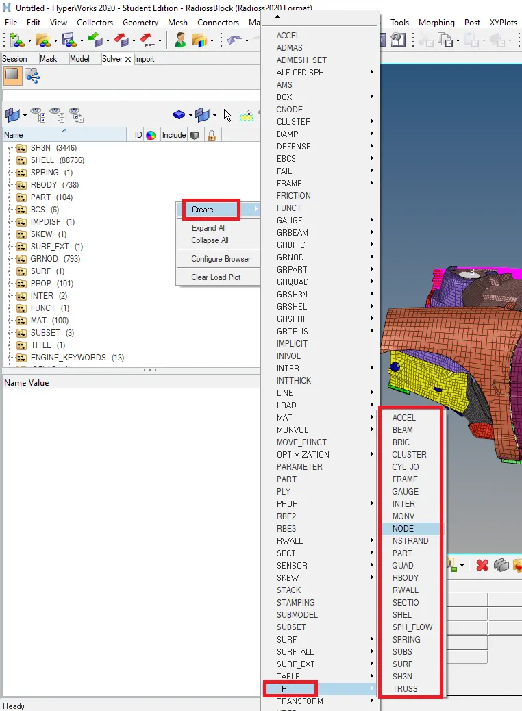
Create -> Time History
Then after creating a TH for one type, we then simply need to give the entity on which we need the TH to be plotted.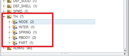
All the TH defined
These are all the Time-History Output requests that we can request in this case. So, for example, in the Spring TH, we can give the entity as the Spring in the Impactor.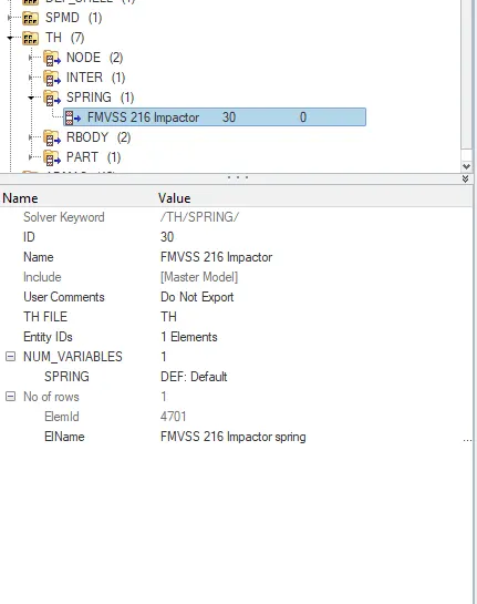
Example for a TH defined
9. After the Deck Setup is done, the last step includes checking the model in the Model checker. To check the model, we can use the Model checker in either Hypermesh or Hypercrash. In Hypermesh, the Model checker can be accessed under the Tools tab.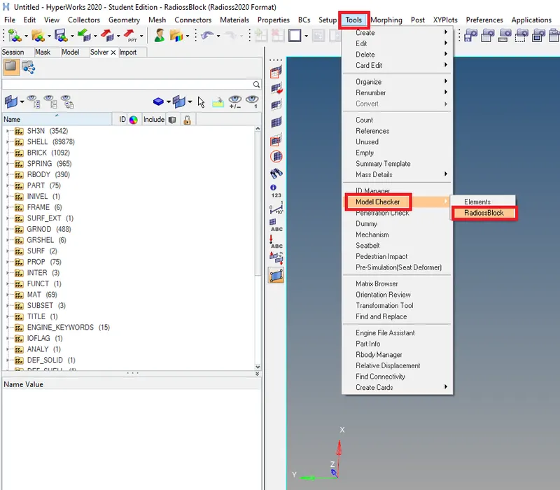
Tools -> ModelChecker
This model checker will show all the warnings and errors in the model. All the errors must be resolved and the warnings if not critical, can be left in the simulation, else, they too must be resolved. Like this the model can be checked and be resolved for any errors in the model.
After the model checker is run, we then go on to run the simulation. To run this simulation we have to use the Radioss command in the Analysis tab.
Analysis -> RADIOSS
RADIOSS Command
The input file is the file location in the system where we want to save all the simulation files, such as the .h3d file and the T01 files for example.
After the simulation is run, we can confirm that the simulation has run properly when we see a NORMAL TERMINATION at the end of the simulation as follows: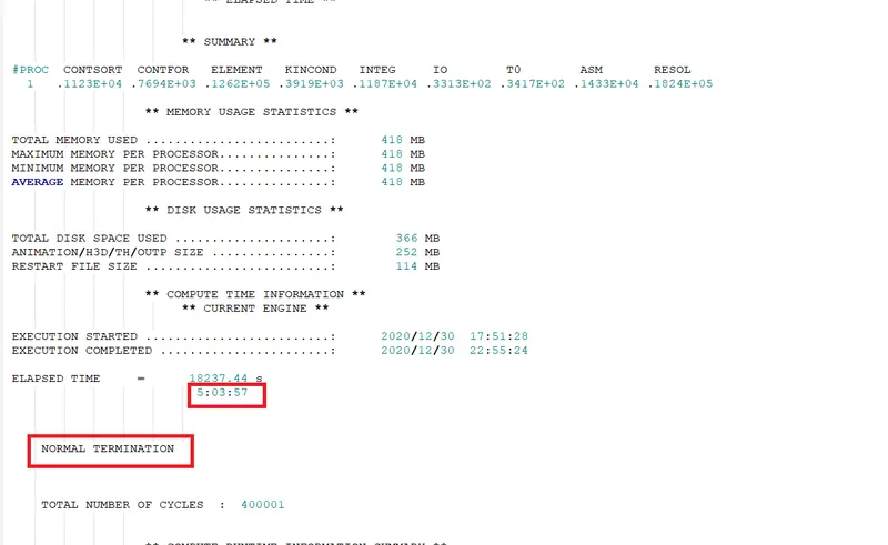
Normal Termination and Elapsed Time
The Elapsed time is approximately five hours and four minutes in our case.
We can then later view the simulation in Hyper-view.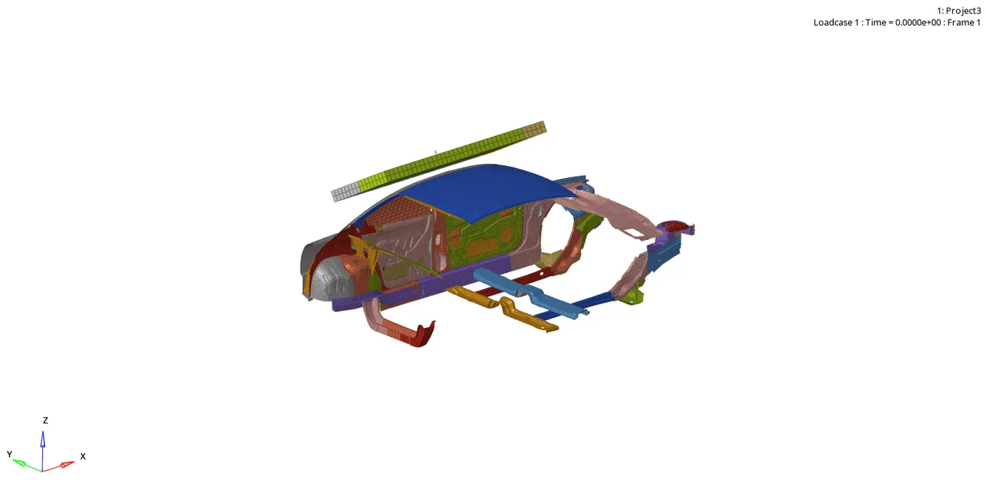
Animation of the Simulation.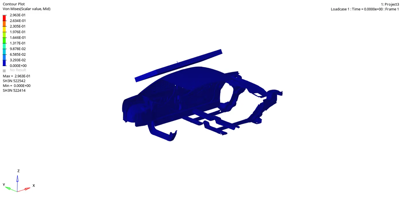
Von-Misses Plot.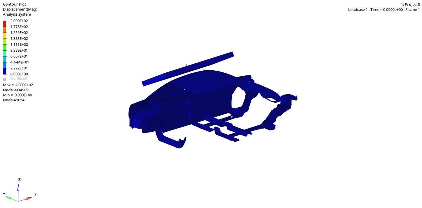
Displacement Plot.
10. The very last step is to study the Simulation results by plotting all the necessary graphs and extracting data from them. To plot graph, we need to use the Hypergraph tab. To access the Hypergrraph tab, we simply need to change as the following: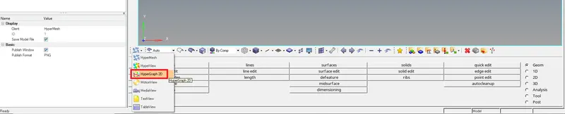
Hypergraph 2D
In this tab we need to open the Time history file. It is the T01 File that will be available in the Folder where we saved all the files. We can import this file by clicking on the icon shown below:
HyperGraph Command
We can set the variables between which we need the graph to be plotted as well.
A. Energies of the Simulation:
A.1. Total Energy and the Internal Energy: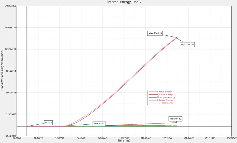
Energies Plot
Ideally: Hourglass Energy+Contact Energy / (Total Energy) ≤15%
In our case:
(0 + 101.82) / 2346.18 = 4.33%
This is well below the limit, hence this condition is satisfied.
From the above plot, we can see that the Internal Energy is continuosly increasing, this can mean that the Deformation in the elements is continuously increasing in the simulation. Ideally all of KE should be converted into IE and the Total Energy must remain constant.
On careful examination, we can plot the low scale graph as following: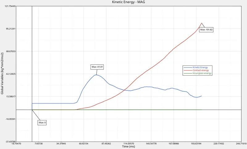
We can compare the simulation with the Graph and we can observe that both the Kinetic Energy and the Contact Energy are increasing from the moment that the Impactor makes contact with the Roof. The increase in the Contact Energy can be justified because, it is the energy that our contact algorithm uses to push the slave node away from the master node. The increase in Kinetic Energy can be justified because the impact causes the some motion in the elements which then results in the increase in the Kinetic Energy.
As for the hourglass energy, we have gotten a zero value for it, meaning that there was no Hourglass Error in the simulation.
Our Requirement from an Ideal Simulation is that we have minimal Contact energy and maximum Energy absroption/Deformation in the elements. We can check the Energy error in the Engine output file, which has maxed out at -4.1% which is also within the appropriate limits for it to be. Our Mass error is also 0.26% which is also within the limits for it.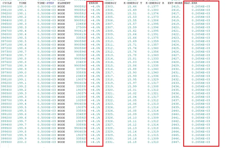
Engine Output file.
B. Contact Interface Forces.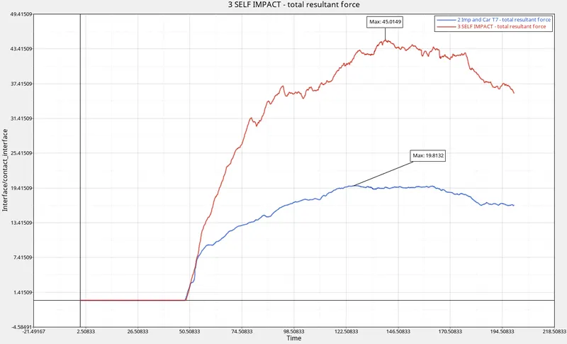
Contact Interface forces plot.
In the Plot above, we can see that the Self impact contact interface has a peak higher than the Contact interface defined between the Car and the impactor. The Self impact contact has a force of 45.0KN whereas in the case of the contact between Car and the impactor, it has a peak force of 19.8KN.
C. Animation Output
1. Plastic Strain: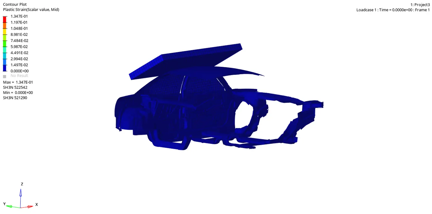
Plastic strain can be defined as Strain developed in a deformed body in which the distorted body does not return to its original size and shape after the deforming force has been removed. When we compare these data with the lab data(SigY), we see that we get this value higher than then Yield Stress, hence we can confirm that the entire model is in Plastic Region.
2. Hourglass energy
Since there was no Hourglass Energy Error in the simulation(can be confirmed with the graph plotted), no such animation changes can be seen in the above simulation.
3. Specific Energy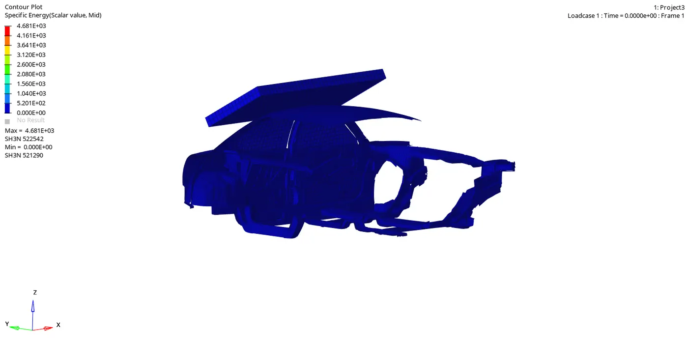
Specific Energy can be defined as the Energy per unit mass. Specific Energy is an Intensive Property. The higher the energy density of a system or material, the greater the amount of energy stored in its mass. In scientific equations, energy density is often denoted by U. The maximum magnitude of our Specific Energy that we have gotten is 4.7KJ/kg.
D. Force vs Displacement Plot.
To plot a Force vs Displacement graph, we need to use the option of Cross Plot. To activate the Cross plot option, we must use the preference File setting and use the Vehicle Safety Standards option in it.
To build a cross plot, we must have a Plot of the Force vs time of the contact interface between the Impactor and the car. And the second plot that we need is the Displacement of any one of the nodes on the car. To do this, we must build plots of that node in a separate window. Now in the third window, we must use the cross plot option and select (Shift+curve select) the displacement curve in the X-axis and the Force in the Y-Axis and create the plot.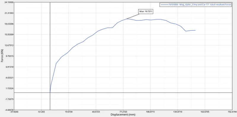
Force vs Displacement Plot.
From the plot above, we can see that the maximum Force that we get is 19.73KN at around 80.0mm displacement of the master node of the Rigid body of the Impactor in the simulation.
To check if the FMVSS 216 target load of 47,000 N (= 3 * GVW) has been met, we must know the Gross Vehicle Weight (GVW) of our model. In our case, it is 700kg. To now convert this into weight, we must multiply it by 9.81, then we get 6867N. And, as a Factor of Safety, we multiply this value by 3 and get the Target load as 20,601N.
Since our value is lesser than the specified value of 47,000N, we can conclude that the this condition has been satisfied and met properly.
- Conclusion: In conclusion, I would like to state that this project helped me get a proper understanding on the procedure of analysing the Roof Crush Impact of a vehicle and how to extract different data from the simulation.