Rayleigh Taylor Instability

Rayleigh-Taylor Instability

Introduction

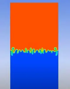
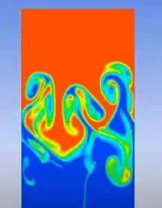
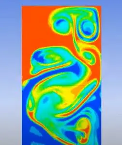
Rayleigh-Taylor instability is an instability that occurs at the interface of a mixture of two fluids of different densities. In case a heavier fluid rests atop a lighter one, under the influence of gravity it moves downwards, while the lighter fluid moves upwards, as shown in the figure below.

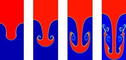
Examples: Water and oil mixture and plasma fusion reactors.

Objectives

1. To describe some practical CFD models that have been based on the mathematical analysis of Rayleigh-Taylor waves.
2. To perform simulations of the RT instability using meshes of different sizes and to discuss the results.
3. To define the Atwood number.

Theory description

Practical models used:

1. Plateau Rayleigh-Taylor Instability: Explains how a falling stream of fluid breaks up into smaller packets with same volume but lesser surface area. Used in design of inkjet technology. (inkjet printing)
2. Kelvin-Helmholtz Instability: A sporadic and widespread phenomenon that usually occurs in atmosphere. Seen in the flow of wind over water and is also often invisible, such as clear air turbulence and hence can be very dangerous. It occurs when two fluids flow over each other at different velocities such that there is a discontinuity at the interface.

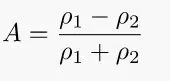
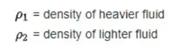
Atwood Number: It is a dimensionless number used to describe hydrodynamic instabilities in flows involving fluids of two different densities.

Methodology

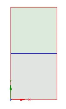
A simple two dimensional geometry is modelled using Ansys spaceclaim to simulate the Rayleigh-Taylor Instability.

The denser fluid is placed in the upper region, where as the lighter fluid in the lower.

Share topology has been enabled to define the interface between the two fluids.

Viscous model used is laminar

A Transient solver is used as the flow is to be observed at every instant, and the properties of flow at each point change with respect to time.

Every simulation was run for 500 time steps, at a time step size of 0.005 s.

Baseline mesh:

The fluid at the top is water, while the fluid at the bottom is air.

A mesh has been created using element size of 0.5 mm

Next, two more flow simulations are performed using mesh of sizes 0.3 mm and 0.2 mm.

0.3 mm mesh size:

0.2 mm mesh size:

Atwood number is calculated as: (1000-1.225)/(1000 + 1.225)

A = 0.99

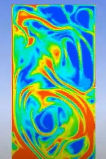
A new fluid having density 400 kg/m3 is also simulated with water, using a mesh size of 0.2 mm:

Atwood number = (1000-400)/(1000+400)

A = 0.43

Inferences and Results:

• Using a finer mesh gives a more accurate and visualizable flow. The bubble formation is more clearly seen in the refined cases as compared to the baseline mesh.
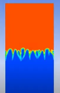
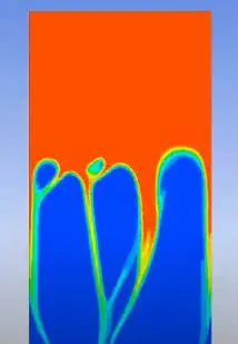
• Coming to the Atwood number, a value closer to 1 involves more bubble like formation at the inital interface, whereas a lower Atwood number leads to the formation of finger like projections initially at the interface.

Atwood Number 0.99

Atwood Number 0.43