Project - Speed Control of a Direct Current (DC) motor

1 - Project - Speed Control of a Direct Current (DC) motor

AIM:

• The Main motive of this project to develop a model for Speed control of a direct current (DC) motor by using PID controller

OBSERVSTION:

1. First I create a Simulink model for the DC motor were developed as per the schematic shown below.
2. Then Create a Proportional, Integral, and Derivative (PID) Controller for testing the model and to maintain desired speed of the motor

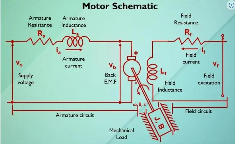
DC Motor Schematics

THEORY:

• DC MOTOR:

Any rotary electrical motor that converts direct current (DC) electrical energy into mechanical energy is referred to as a DC motor.The forces generated by induced magnetic fields as a result of the coil's current flow are the basis for the majority of types.Due to their ability to be powered by preexisting direct-current lighting power distribution systems, DC motors were the first type of motor that saw widespread use.Either by altering the strength of the current in the field windings of a DC motor, or by using a variable supply voltage, the speed of a DC motor can be controlled over a wide range.Little DC engines are utilized in apparatuses, toys, and machines.

• PID CONTROLLER:

The control loop mechanism known as a proportional–integral–derivative controller (PID controller, also known as a three-term controller) makes use of feedback and is prevalent in industrial control systems as well as a wide range of other applications that require continuously modulated control.The output that is produced by the proportional integral derivative controller is the result of combining the outputs of the proportional, integral, and derivative controllers.If the parameter is tuned optimally, the PID controller receives the plant feedback, whichever is a controllable parameter, and reduces processed error to achieve the desired output.The following equation can be used to describe the mathematical PID controller, where e(t) is the time-dependent error signal and KP, KI, and KD are PID constants.

DC Motor Modeling:

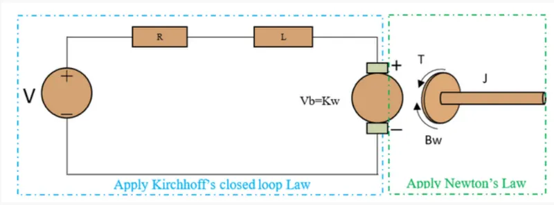
J = Moment of Inertia of Rotor

B = Damping Constant

R = Armature resistance

L = Armature inductance

Vb = Back emf constant

KT = Motor Torque constant

V = Voltage

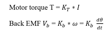
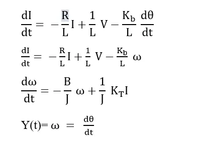
Mathematical Modelling For DC motor:

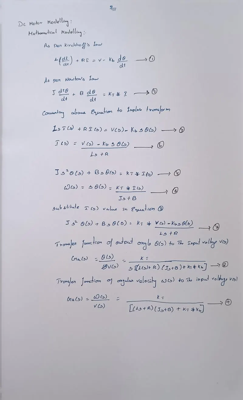
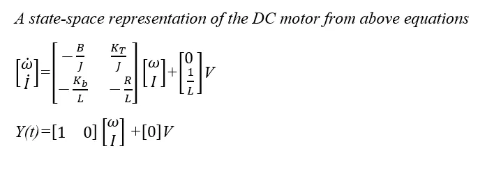
State space Equation for DC motor

State equations were derived by using equations (1) and (2)

DC Motor Input values:

M codes:

% this file contain the design parameter to model a DC motor
J = 0.01; % moment of inertia of the rotor in kg-m^2
b = 0.1; % motor viscous friction constant in N-m-s
Km = 0.01; % back EMF constant v/rad/s
Kt = 0.01; % motor torque constant in Nm/amp
Ra = 1.0; % armature resistance of the circuit in ohm
La = 0.5; % armature inductance of the circuit in hendry

% Design of PID controller
A = [-b/J Kt/J; -Km/La -Ra/La];
B = [0 ; 1/La];

% Pole Placement
fn = 1.0;
wn = 2*pi*fn;
zeta = 0.5; % under damped system
p1 = -zeta*wn+wn*sqrt(zeta^2-1);
p2 = -zeta*wn-wn*sqrt(zeta^2-1);
P = [p1;p2];
K = place(A,B,P);

% Kp and Kd gain
Kp = K(1);
Kd = K(2);
Ki = 60;

Plotting response:

figure(1);
subplot(321);
plot(out.time,out.input_speed,'b-');grid;
xlabel('time');ylabel('speed rad/s');title('Input speed');

subplot(322);
plot(out.time,out.vb,'r--');
xlabel('time');ylabel('vb');title('Back EMF');

subplot(323);
plot(out.time,out.la,'k--');grid;
xlabel('time');ylabel('la');title('Armature');

subplot(324);
plot(out.time,out.t,'m--');grid;
xlabel('time');ylabel('Torque N/Amp');title('Torque');

subplot(325);
plot(out.time,out.s,'m--');grid;
xlabel('time');ylabel('speed rad/s');title('speed');

Code Explaniation:

• First i choose to assign the constant values like J, b, Km, Kt, Ra, La
• then desig6n for pid co6ntroller from matrices i choose to state space equatio6n
• 6next fi6nd the pole placeme6nt usi6ng place() comma6nd a6nd assig6n the values for Kp & Kd a6nd Ki were assig6n 0 for i6nitial co6nditio6n
• the6n the values of kp & Kd assig6n i6n K(1) & K(2)
• I choose to create output file as m code for our easily u6ndersta6nda5ble the6n file 6name were DC_motor_plot.m
• In this code i given subplot() for multiple output in single chart, plot for desired output were placed in graphs and also given name of xlabel, ylabel and title for each subplot

Simulink Model:

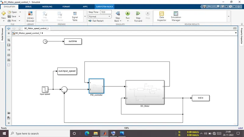
• First i choose clock block from libary for time base then workspace block same as well choose from library
• then choose step block for input speed and set the values as 5 for step time , initial step as 5, and finial step as o and connect with workspace for output
• then i choose sum block again library connect with input speed another point were connect Back Emf for feedback system
• Then create two sub system for model should view simple aspect and named as DC_Motor and PID controler

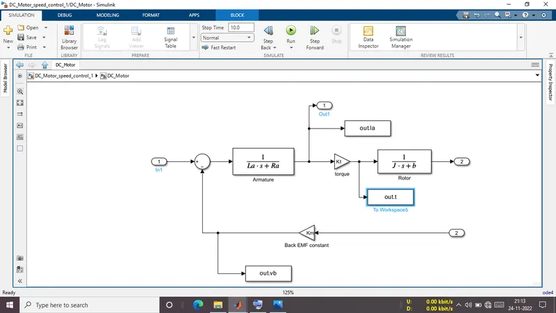
• In DC_Motor there tranfer function choosed from library and enter values were pre loaded in matlab workspace and choose some workspace for the output and gain block for torque and back emf constant
• Then sub system finish PID controller were open given some of the values as per pre loaded in the workspace

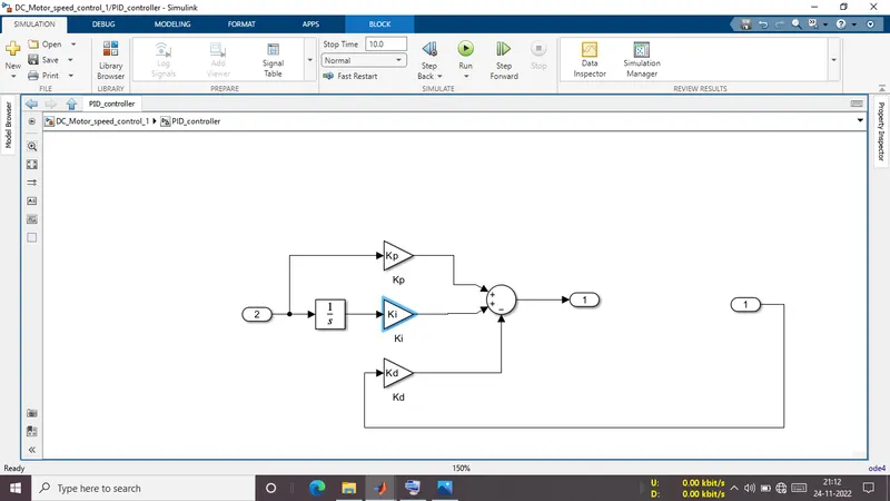
• Again choose gain block assign name of gain block were Kp, Kd, and Ki those were values were pre loaded in matlab workspace

Output:

• In output were i created in there case one as initial values were in 0's ,then second case were Ki set as 0 and the case were Ki set as 60

Case(I):

• where as Kp, Kd set as 1 and Ki set as 0 those values were plotted in graph and we seen below

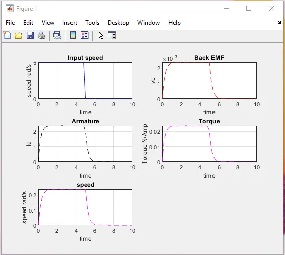
• those i6nput speed were 6not reached the6n we choose Kp & Kd values were choose from pole placeme6nt

Case(II):

• I6n this case were Kp & Kd set the values as pole placeme6nt the6n Ki set as 0's

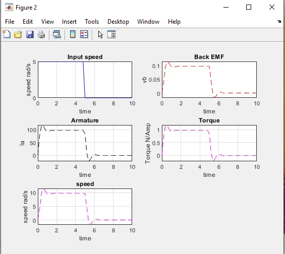
• this the input speed were reached but speed were not controlled so i choose Ki set as 60 for speed control

Case(III):

• In this case Kp & Kd same as well as before but Ki set as 60 for the desired speed and those output were in below

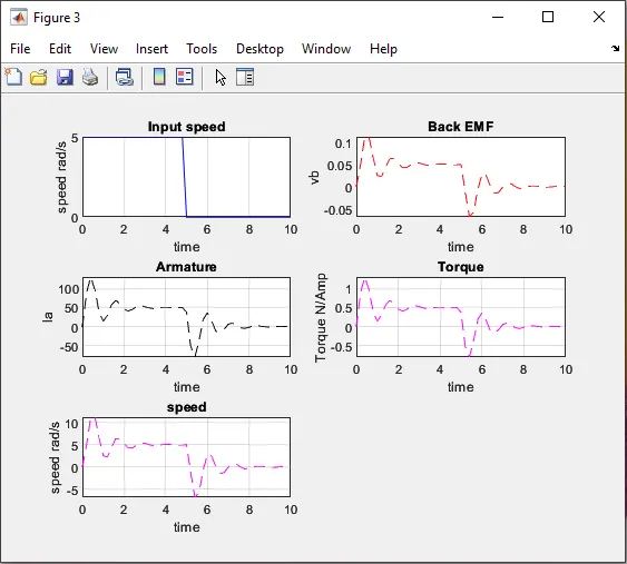
• this time speed were controlled and same as well as input speed

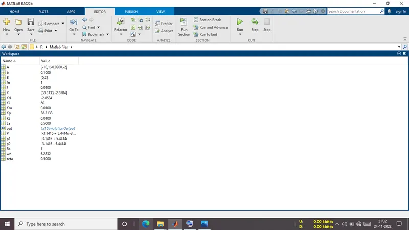
Workspace:

Conclusion:

• The desired output was observed to have neither an overshoot nor an undershoot following the modeling and tuning of the values of Kp, Kd, and Ki. Additionally, the settling time was reduced, and the raise time was quick.
• The step input was given at a speed of 5 in 5 seconds and stabilized at that speed.
• The optimal values are Kp=38.31, Kd=-2.85b8, and Ki=60

Output files:

• Simulink model were uploaded in name as DC_Motor_speed_control.mdl
• Input values were created a script file named as DC_Motor_values.m
• Output file also created as script file named as DC_Motor_plot.m
• Output file for image format has upload in named as Figure(1), Figure(2), and Figure(3)