PID Controller Desgin For DC Motor:
The Proportional, Integral, and Derivative (PID) control design knowledge gained to design, develop and test a controller to maintain a desired speed for the motor.
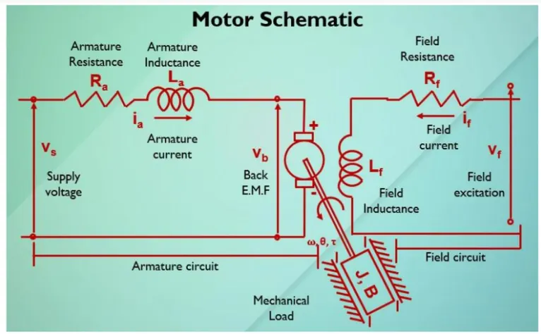
# Mathematical modeling from the principles:
- using krichhoff's voltage law ,
Vs = Ra*ia + La (dia/dt) + Vb
- Back EMF, angular velocity and torque are related by
Vb = Km (d`theta`/dt) T = Kt*i
here, Km and Kt are the back EMF and torque constant respectively
- Angular velocity
w = `theta`dot
- The open_loop transfer function for the motor with the speed (w) and supply voltage(Vs) can be derived as
w(s) / Vs(s) = Kt / (J*La*s^2) + (J*Ra+B*La) s + (B*Ra + Kt*Km)
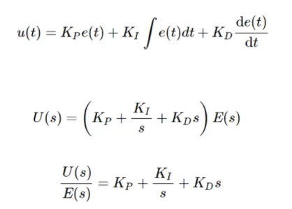
- A PID controller design is obtain the desired angular speed using the appropriate supply voltage
-Mathematically PID controller can be defined by the following
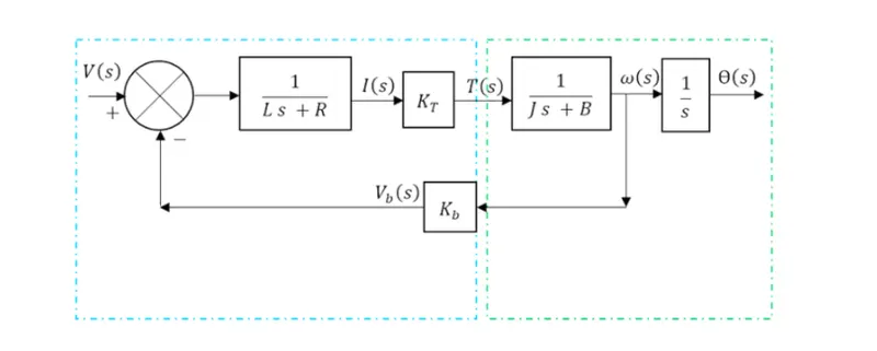
# Modeling of dc motor:
I(s) = V(s) - Kb*s*θ(s) / Ls + R w(s) = S*θ(s) = Kt*I(s) / Js+B
# PID Design for speed CONTROL OF DC motor:
% This file contains parameters for DC motor design
J = 0.01; % Inertia
b = 0.1; % friction
Km = 0.01; % back emf
Kt = 0.01; % torque
Ra = 1; % resistance
La = 0.5; % inductance
% Design of PID controller
A = [-b/J Kt/J; -Km/La -Ra/La];
B = [0 ; 1/La];
% Placement of Poles
fn = 1;
wn = 2*pi*fn;
zeta = 0.5;
p1 = -zeta*wn+wn*sqrt(zeta^2-1);
p2 = -zeta*wn-wn*sqrt(zeta^2-1);
P = [p1;p2];
K = place(A,B,P);
Kp=K(1);
Kd=K(2);
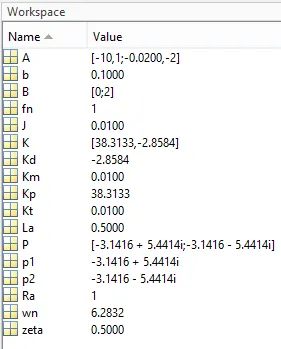
- The output values for the above script:
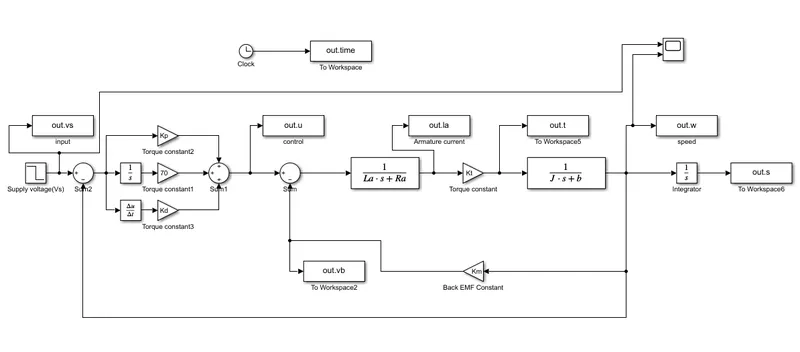
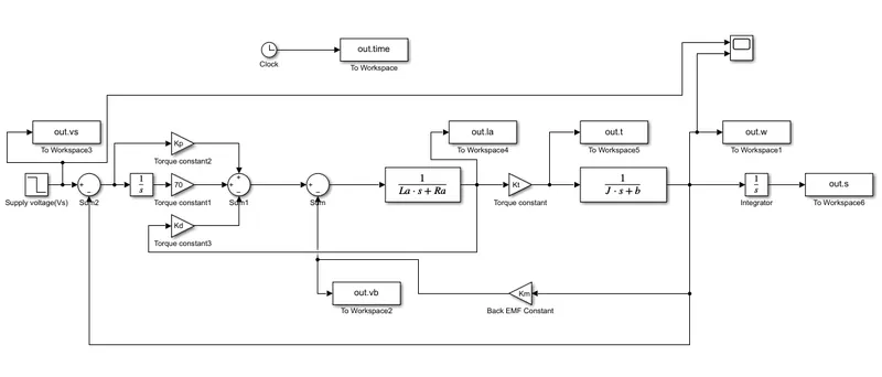
#SIMULINK BASED MODELING:
- Speed error signal as feedback feedback for gain Kd:
- Armature current feedback with gain Kd:
#Control law design :
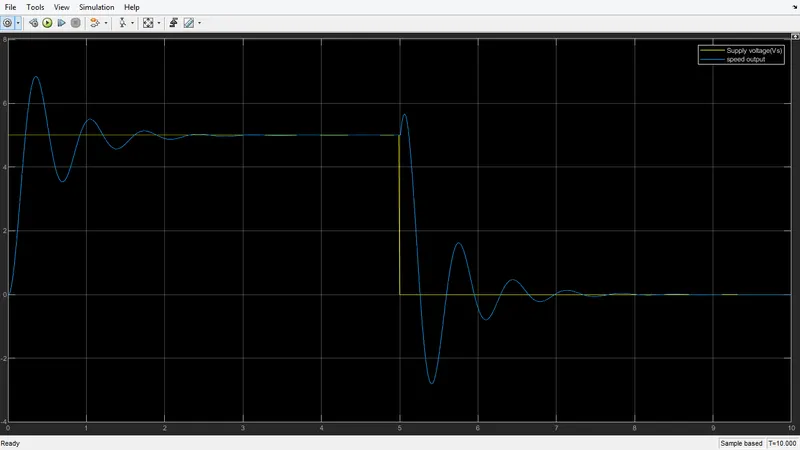
- Setling time < 3s
- Overshoot < 15%
- Steady state error < 1%
# OUTPUT RESULT:
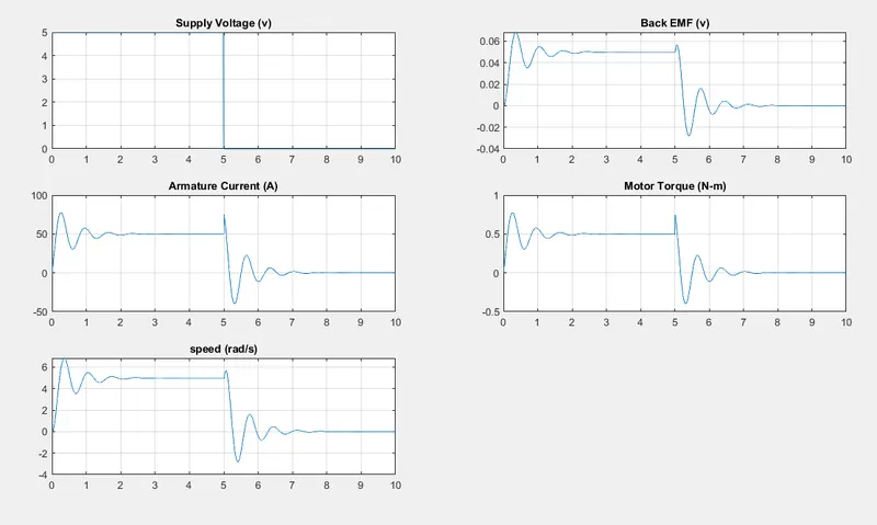
- DC Motor plot:
close all;
subplot(321);plot(out.time,out.vs);grid;title('Supply Voltage (v)');
subplot(322);plot(out.time,out.vb);grid;title('Back EMF (v)');
subplot(323);plot(out.time,out.la);grid;title('Armature Current (A)');
subplot(324);plot(out.time,out.t);grid;title('Motor Torque (N-m)');
subplot(325);plot(out.time,out.w);grid;title('speed (rad/s)');
#Control law Test:
Ki = 70 we getting required design.
- Setling time < 3s
from above result we can find the settling time is less then 3s asper the design we already create.
- Overshoot < 15%
from the result we can say overshoot is less then 15%.
- Steady state error < 1%
steady state error is less then 1% from the above scope we can find.
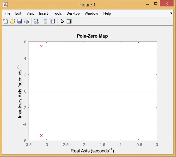
#Stability of a dynamic system:
script:
k_dc =1; % DCgain of the system is 1
s = tf('s');
G1 = k_dc*wn^2/(s^2 + 2*zeta*wn*s + wn^2);
pzmap(G1,'r')
We can see two crosses in red indicate complex poles lying on the left hand (negative side) of the plane which indicate it is a stable system.