Project - Speed Control of a Direct Current (DC) motor
PID Controller for speed control of d.c. motor (Project Report)
Simulink model & results
A motor is a machine that convrts electrical energy into mehanical energy.The d.c. motor is a very similar to the d.c. generator in construction. Generators are generally operated in more protected locations & therefore their construction is open type but the motor are used in locations where they are exposed to dust,moisture,fumes & mechanical damage, so it adversly affect on the speed of motor also. To regulate the speed of a motor, there are various method to control it, but we want to develope a simulink for the regulation of speed of d.c.motor using Proportional-Integral-Derivative(PID) controller by appropriate choosing the values of control design like rise time, settling time, overshoot & steady state error. Figure 1 shows the equivalent circuit diagram of d.c. motor.
Figure 1. Equivalent circuit diagram of d.c. motor
The mathematical equation for d.c. motor is given by,
Vs= Ia*Ra + L*(dIa/dt) + Vb
Ia*Ra + L*(dIa/dt )= Vs-Vb ------------------------------------------------- ---(I)
Where Vb = Kb*w = Kb*( dθ/dt)
J*(d2θ/dt2) + B*(dθ/dt) = KT*Ia --------------------------------------------(II)
Convert the above equation in Laplace ‘S’ domain
I(S)*R + L*S*I(S) = V(S) - Kb*I(S)
I(S) = (V(S) - Kb*I(S)) / (L * S + Ra) --------------------------------------------------(III)
J* S2 * θ(S) + B*S* θ(S) = KT*I(S)
S * θ(S) *[J * S+ B] = KT*I(S)
S * θ(S) = KT* I(S) / [J * S+ B] or W(S) = KT* I(S) / [J * S+ B] ---------------------(IV)
where, S * θ(S) = W(S)
Substitute the value of I(S) from equation III in equation IV, we get a transfer function as follows:
G(S) = W(S)/I(S) = KT / [(L*S+R)*(J*S+B) + (KT * Kb)]
where,
Vs= d.c. Supply voltage, volt
Ra= Armature Resistance, ohm
L= Armature Inductance, henry
Ia= Armature current, ampere
Vb = Back emf, volt
J = moment of inertia, Kg-m2
B = motor viscus friction coefficient constant, N-m
T= torque, Nm
Kb= back emf constant, volt/rad/sec
KT= Torque constant,N-m/amp
θ = Output angle, radian
S = Laplace variable
In state space model,
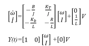
Figure 2 shows the simulink model for above equations,
Simulink model:
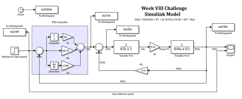
Figure 2. Simulink model for regulating the speed control of d.c. motor
controller we developed :
We have develoed a PID controller shown in figure 3.
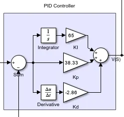
Figure 3. Porportional-Integral-Derivative (PID Controller)
Before developing the PID controller, we have calculated the values of Kp & Kd from following matlab code shown in figure 4. By using place command i.e. k=place(A,B,p), we have found the values of both Kp & Kd. When we run the matlab program, we obained the values of poles P1 & P2, Kp & Kd. This is shown in figure 5.
Matlab code:
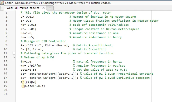
Figure 4. Matlab code for d.c.motor design parameters, PID controller
% This file gives the parameter design of d.c. motor
J= 0.01;                    % Moment of inertia in kg-meter-square
B= 0.1;                     % Motor viscus friction coefficient in Newton-meter
Kb= 0.01;                   % Back emf constantin volt/rad/sec
Kt= 0.01;                   % Torque constant in Newton-meter/ampere
Ra=1.0;                     % Armature resistance in ohm
La= 0.5;                    % Armature inductance in henry
% Design of PID Controller
A=[-B/J Kt/J; Kb/La -Ra/La];  % Matrix A coefficient;
B= [0; 1/La];                 % Matrix B coeffint
% Following data gives the poles of transfer function
% Values of Kp & Kd
fn=1.0;                       % Natural frequency in hertz
wn= 2*pi*fn;                  % Angular frequency in rad/sec
zeta=0.5;                     % set the value of zeta to 0.5;
p1= -zeta*wn+wn*sqrt((zeta^2-1)); % value of p1 i.e.Kp Proportional constant
p2= -zeta*wn-wn*sqrt((zeta^2-1)); % value of p2 i.e.Kd Derivative constant
p=[p1;p2]
k=place(A,B,p)
In this program, we mentioned the values of design parameters such as moment of inertia, motor friction viscous constant, supply voltage, armature resistance, inductance etc. which are required for d.c. motor speed control & also for PID controller
Matlab Output:
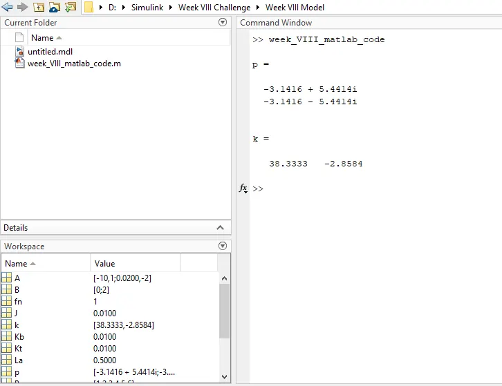
Figure 5. Matlab Output showing values of Kp & Kd
From figure 5, we have seen that the value of K1 & K2 is Kp & Kd, i.e.
Kp=38.33 ; Kd= -2.86
where, Kp = Proportional gain constant;
Kd = derivative gain constant;
Ki = integral gain constant
Now the value of Ki is tunned manually such that the control design parameters like settling time, overshoot & steady state error are met. So, we have set the value of Ki is 65. For this values, we get better control responce.
Now, we want to show the results in a graph with the help of matlab, we have designed another matlab program which is shown in following figure 6.With the help of this program, we can obtain the graph of reference input speed, supply voltage, error signal & angular speed.
Matlab code for showing graph:
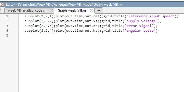
Figure 6. Matlab code showing the graphs
subplot(2,2,1);plot(out.time,out.ref);grid;title('reference input speed');
subplot(2,2,2);plot(out.time,out.Vs);grid;title('supply voltage');
subplot(2,2,3);plot(out.time,out.Es);grid;title('error signal');
subplot(2,2,4);plot(out.time,out.Ws);grid;title('angular speed');
Figure 7 shows the graph of reference input speed,supply voltage, error signal & angular speed. In simulink model, we set the values of reference speed as 100 & supply voltage is 230 volt. Error signal comapre both input reference signal as well as output which is given to the PID controller as a input. angular speed is nothing but the motor output we obained at the end.
Results:
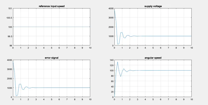
Figure 7. Simulation results
Simulation result:
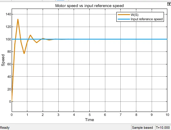
Figure 8. Input & Output speed of d.c. motor
Figure 8 shows the input & output speed of d.c. motor in which blue line indictes the reference input speed which is set to 100 & orange line indicates the controlled speed of d.c.motor i.e. output speed. By comaring both speeds, we have seen that
settling time is near about 1.9 sec. shown in figure 9.
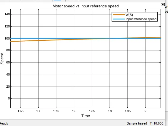
Figure 9. graph showing Settling time set to 1.9 sec
Overshoot is near about 132.46 shown in figure 10.
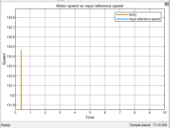
Figure 10. graph showing overshoot set to 132.46
Here there is a negligible steady state error in this result. which is less the 1% shown in figure 11.
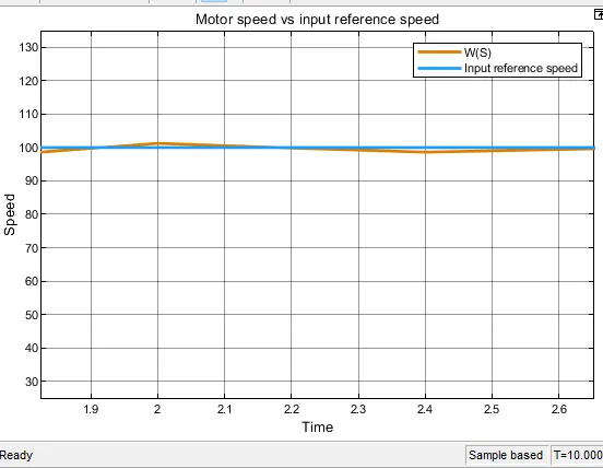
Figure 11. graph showing negligible steady state error
Our main objective is to select the P,I,D gains such that the control design parameters like settling time, overshoot & steady state error are met. So, with the help of above simulink model as well as by selecting the suitable values of P,I & D, we achieved the result as per the requirements.