Project - Position control of mass spring damper system
Solution:
Mass Spring Damper Equation:
f(t)=m*x_dot_dot+c*x_dot+k*x;
Transfer Function for above Equation:
X(s)/F(s)=(1/m) / (s^2+(c/m)*s+(k/m));
Lets compare with Tranfer function Equation,
X(s)/F(s)=K/(s^2+(2*zeta*wn)*s+wn^2);
where,
2*zeta*wn=c/m=100/3.6=27.7778.
wn^2=k/m=400/3.6=111.1111.
zeta=c/2*wn*m=100/75.8946=1.31
zeta=1.31
This is Overdamping System zeta>1.
hence,
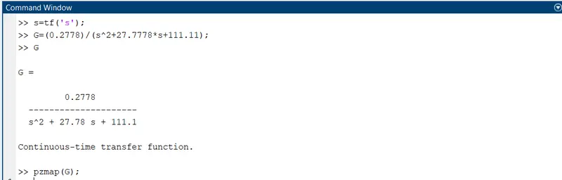
G(s)=0.2778/(s^2+27.7778*s+111.11).
Second Order Equation for mass spring damper system.
x_dot_dot=(f(t)-c*x_dot-k*x)/m
For the above equation design the simulink.
PID Controller Equation:
for PID Controller f(t) is taken as given below.
f(t)=Kp*x1+Kd*x1_dot+Ki*Intergal(x1) dt.
Sub input with reference input So.
x1=x.
x2=x1_dot=x_dot.
x2_dot=x_dot_dot.
apply above assumtion.
f(t)=Kp*(x_ref-x1)+Kd*(d(x_ref-x2)/dt)+Ki*Intergal(xref-x1) dt.
Final Equation:
x_dot_dot=(-c*x_dot-k*x+[Kp(x_ref-x1)-Kd(x2)+Ki(Intergal(x_ref-x1))])/m.
To find State space representation.
x_dot_dot=(f(t)-c*x_dot-k*x)/m.
now take,
x1=x.
x2=x1_dot=x_dot.
x2_dot=x_dot_dot.
Now Consider:
x1_dot=x2.
x2_dot=(f(t)-c*x2-k*x1)/m.
from the above equation to form the Matrix
we get,
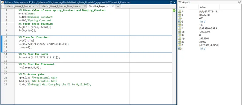
A=[0,1;-(k/m),-(c/m)].
B=[0;(1/m)].
To find the gain from the tranfer equation.
G(s)=0.2778/(s^2+27.7778*s+111.11).
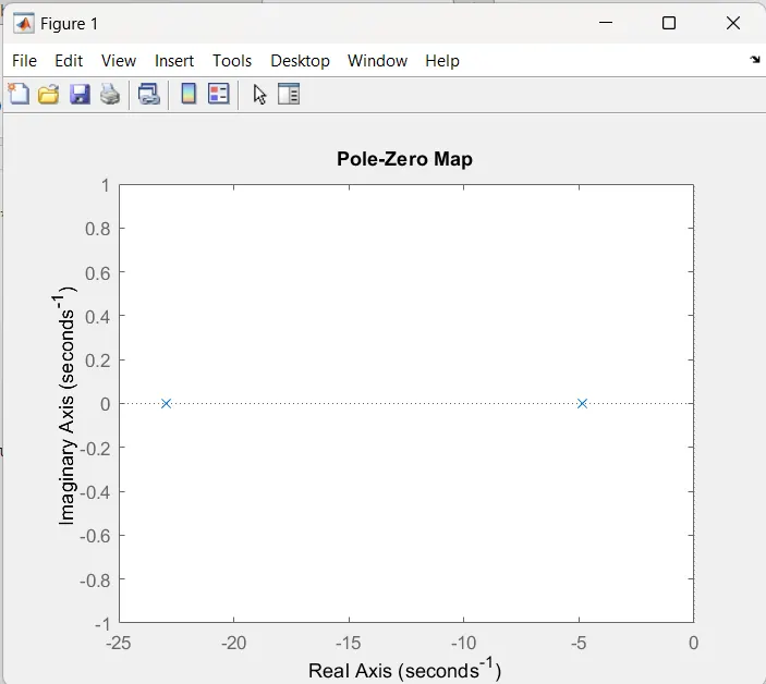
from the use of above equation we can find poles.
P=roots([1 27.7778 111.11]).
P= [-22.9328;-4.8450].
By the uses of A,B,P we can find Placement.
K=Place(A,B,P).
With the help of placement value Propational gain Kp and Derivational Gain Kd is find.
Kp=K(1).
Kd=K(2).
Let assume the Intergal gain Ki according to the system requirement.
Here I assume
Ki=0.
Check poles are stable:
Transfer Function:
pzmap:
Matlab Code:
Simulation Design:
x_dot_dot=(-c*x_dot-k*x+[Kp(x_ref-x1)-Kd(x2)+Ki(Intergal(x_ref-x1))])/m.
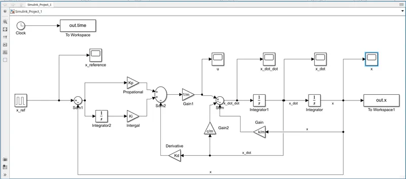
Graph:(Varying Ki value 0,10,100)
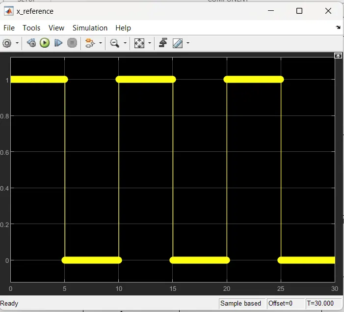
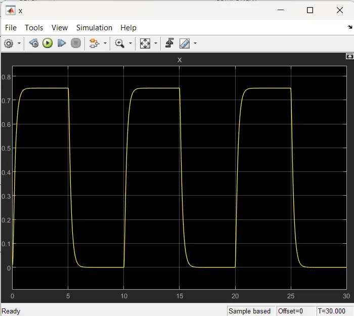
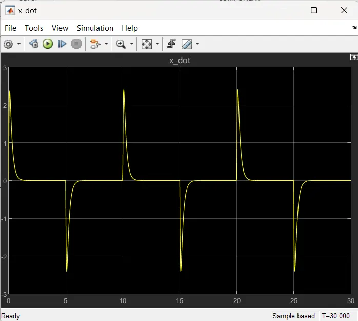
Case 1:
Kp=-22.9328;
Kd=-4.8450;
Ki=0;
x_reference:
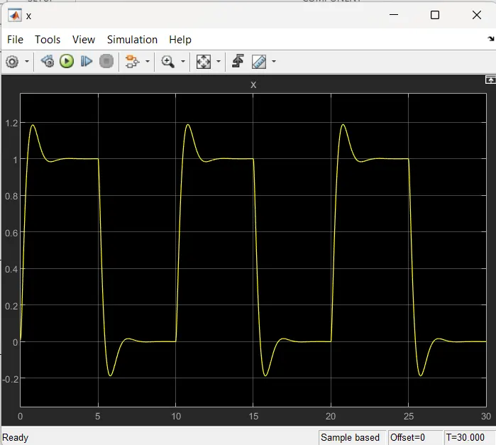
X:
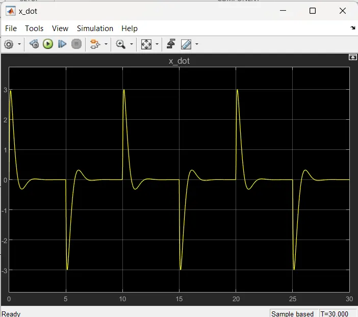
x_dot:
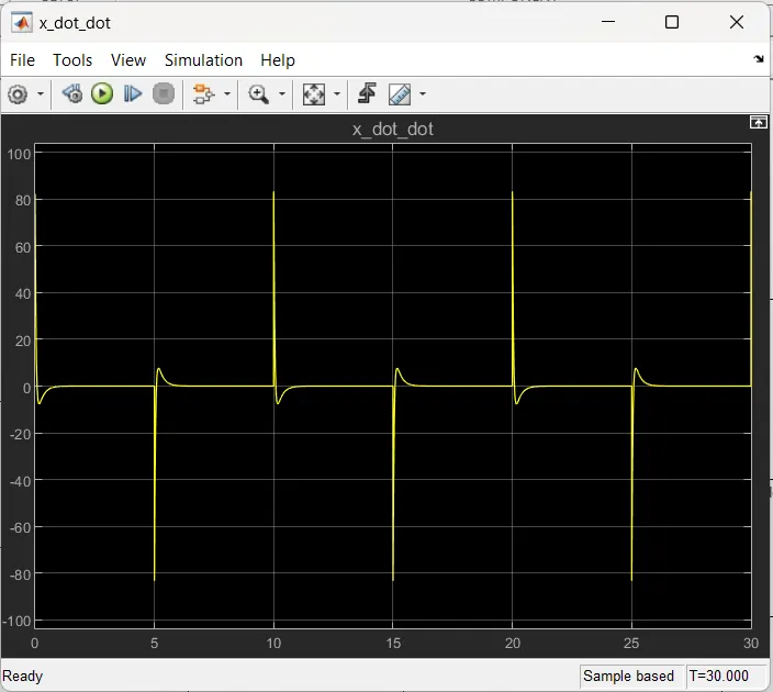
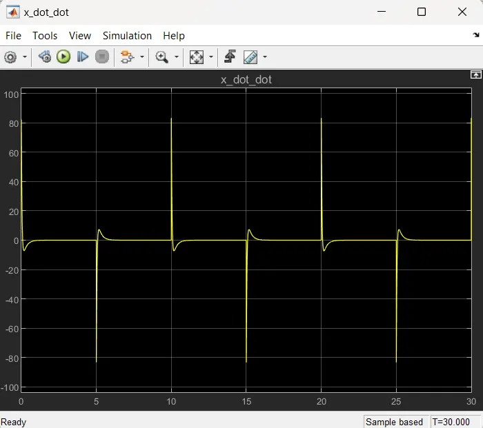
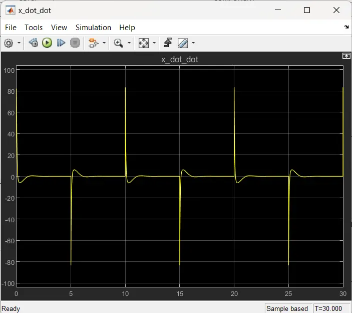
x_dot_dot:
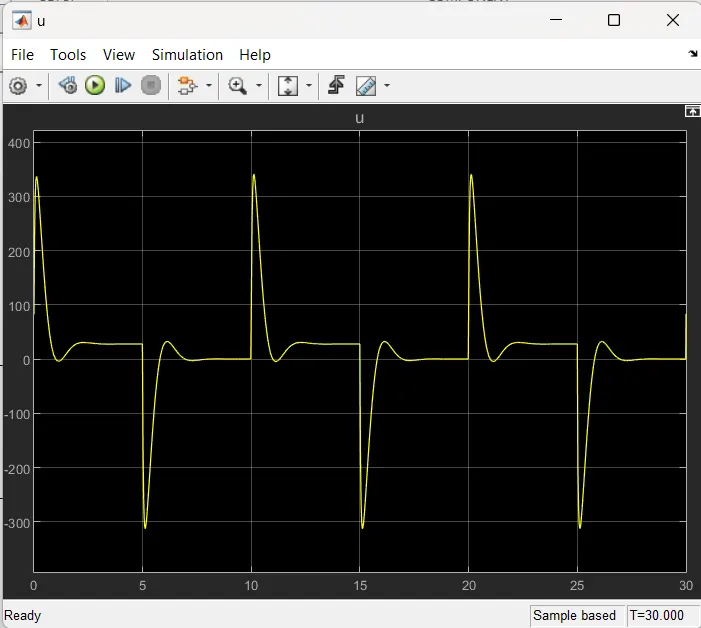
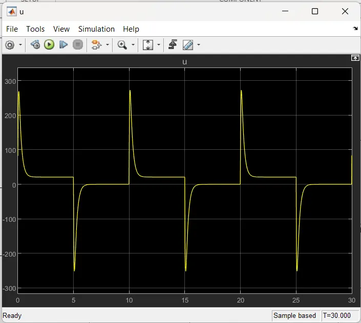
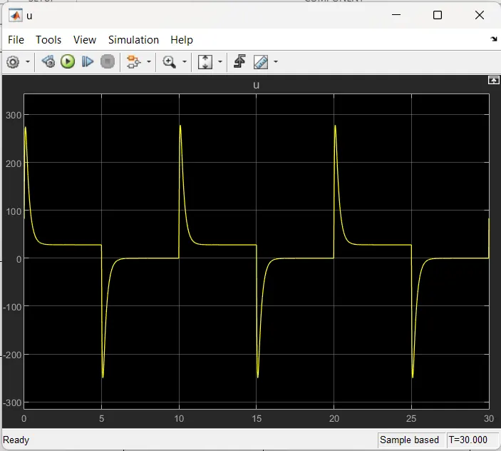
u:
Case 2:
Kp=-22.9328;
Kd=-4.8450;
Ki=100;
x_reference:
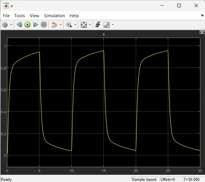
x:
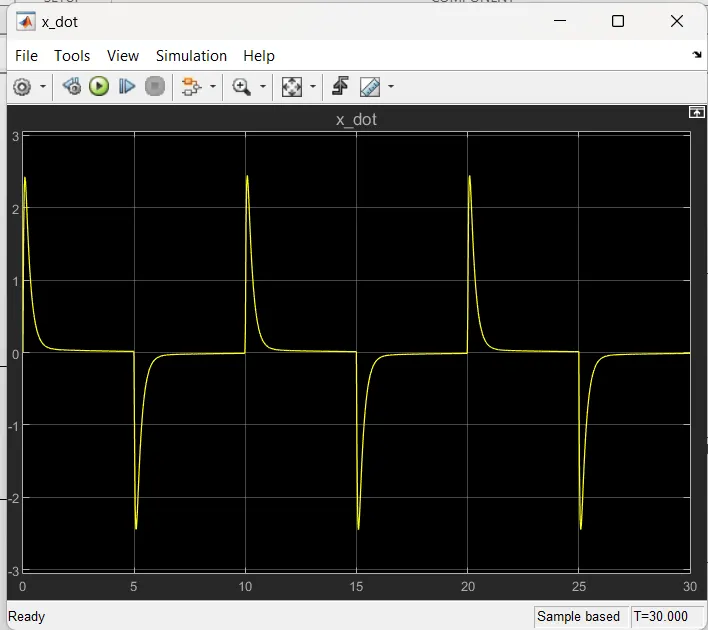
X_dot:
x_dot_dot:
U:
Case 2:
Kp=-22.9328;
Kd=-4.8450;
Ki=1000;
x_reference:
x:
x_dot:
x_dot_dot:
u: