Project - Position control of mass spring damper system

1. Obtain the transfer function of a mass spring damper system and use it in the model. Add a PID controller to adjust the force on mass so that its position follows a reference signal.

Take m = 3.6; %kg k = 400; %N/m c = 100; %Ns/m

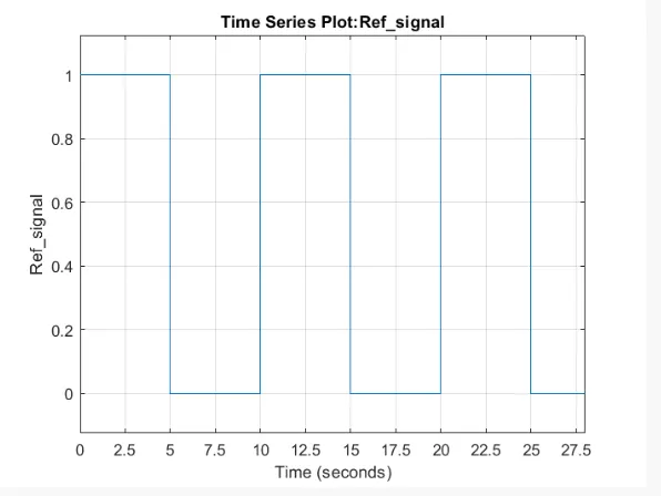
The reference signal is shown in the following figure.

Matlab Code

This Matlab code can set the parameter used in the Simulink model. It also defines the transfer function G(s) and checks the stability of the system

% Parameters for the mass_spring_damper model

m = 3.6;      % mass of the system in kg
k = 400.0;    % spring constant/ stiffness coefficient in N/m
c = 100.0;    % damping coefficient in Ns/m


s = tf('s');             % Laplace transform variable
G = (1/(m*s^2+c*s+k));   % Transfer function of the system

pzmap(G); % Checking the stability of the system
grid on;

wn = sqrt(k/m);     % natural frequency in rad/s
zeta = c/(2*wn*m);  % Damping ratio for an underdamped condition
fn = (2*pi)/wn;     % natural frequency in Hz

%poles are

p1 = -zeta*wn+wn*sqrt(zeta^2-1);
p2 = -zeta*wn-wn*sqrt(zeta^2-1);
P = [p1;p2];

% Pole placement design

A = [0 1; -k/m 0]; %state matrix
B = [0; 1/m];      %input matrix
K = place(A,B,P);  %computing state feedback matrix

% The Proportional, Integral and Derivative Gains are;

Kp = K(1);
Kd = K(2);
Ki = input('Set a value for the Integral gain(Ki): ');

Stability of the System

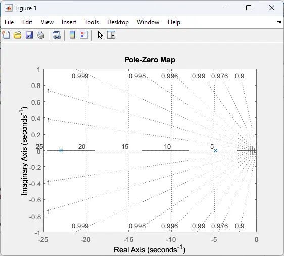
By plotting the poles it is clear that the poles are located at the left-hand side of the imaginary axis, so it is clear that the system is stable.

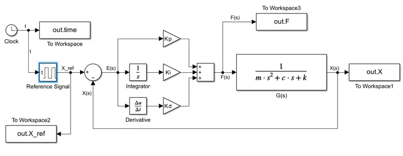
Simulink Model

The mass spring damper system is represented by the following equation;

`f(t)=mddotx+c dotx+kx`

were,

`m=`Mass in Kg

`c=`Damping Coefficient

`k=`Spring constant/Stiffness coefficient

`ddotx=`Accelearation

`dotx=`Velocity

`x=`Displacement

taking Laplace transform on both the sides

`F(s)=mX(s).s^2+cX(s).s+kX(s)`

`F(s)=X(s)[ms^2+cs+k]`

`(X(s))/(F(s))=1/[ms^2+cs+k]` this is the transfer function of the system

from this;

`X(s)=(F(s))/[ms^2+cs+k]`

This equation is used for the Simulink Model.

PID Controller

The PID Controller;

`u(t)=K_pe(t)+K_iinte(t)dt+K_d(d(e(t)))/dt`

Taking Laplace transform on both sides;

`U(s)=K_pE(s)+(K_iE(s))/s+s.K_dE(s)`

`U(s)=E(s)[K_p+(K_i)/s+sK_d]`

`(U(s))/(E(s))=K_p+(K_i)/s+sK_d`

PID Controller Objectives

Setting Time `T_s<2s`

Overshoot `<5%`

Steady State Error `E_(SS)<1%`

Logic

1. The Reference signal is subtracted by the output to generate an error signal.
2. The error signal is fed to a PID controller of Kp, Ki and Kd Gains.
3. The output from the controller is the forcing function.
4. The forcing function is multiplied by the transfer function as per the equation.
5. The generated output from the transfer function block is fed back to the reference signal for subtraction.

Blocks Used

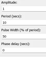
1. Pulse signal: To generate a pulse signal as a reference signal with an amplitude of 1.0 and with a duration of 30.0 seconds.
2. Transfer Function: To execute a Matlab function.
3. Gain: To multiply gain to a signal.
4. Sum: Used to add or subtract input signals.
5. clock: As a time source.
6. To workspace: To store the simulated data in works space.

Input

features of the input pulse signal;

Simulink Model

Output

Matlab Code(for plotting)

figure(1);
subplot(211);
plot(out.time,out.X_ref);
hold;
plot(out.time,out.X,'r--');grid;
title('X_r_e_f & X');
xlabel('Time(s)');
legend('X_r_e_f','X')
subplot(212);
plot(out.time,out.F);grid;
title('Control');
xlabel('Time(s)');

The output which was obtained when using Kp=0.0, Kd=100.0 (obtained from pole placement command) and Ki=500.0(set manually) :

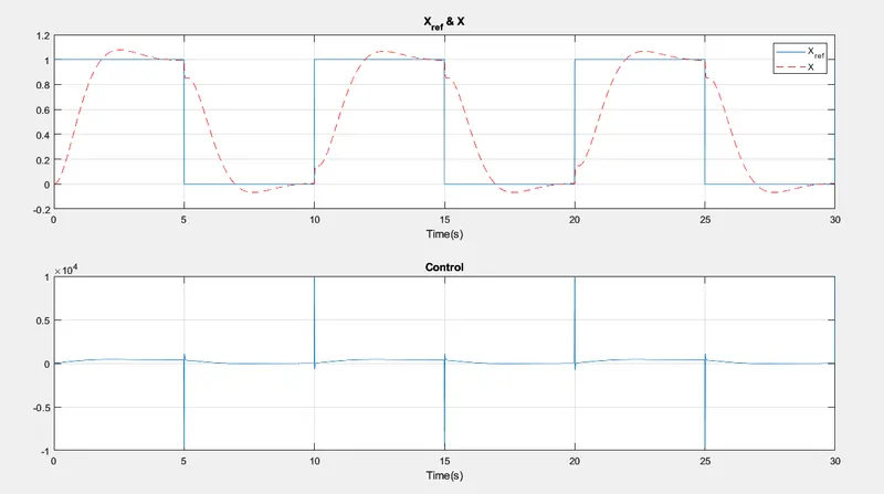
But the output is not excellent in terms of tracking the reference signal (X_ref) and didn't meet the controller objective, so we have to tune the gains manually.

The output which was obtained when using Kp=7000.0, Kd=500.0 and Ki=5000.0(all are set manually) :

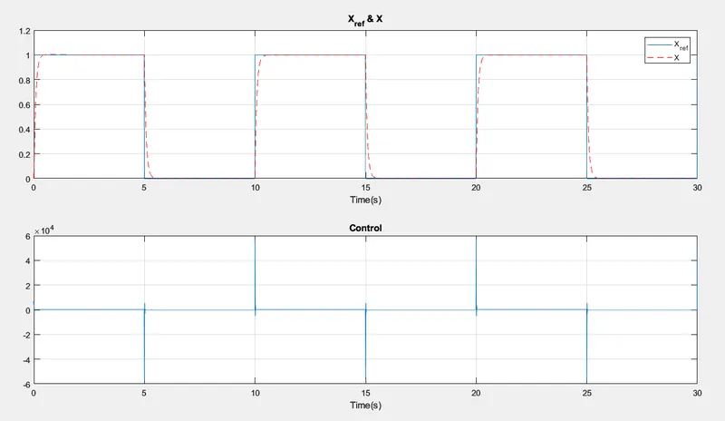
Conclusion

Obtained the transfer function of the mass-spring-damper system and used it in the model. Added a PID controller to adjust the force on mass so that its position follows a reference signal.Taken m = 3.6 kg k = 400 N/m c = 100 Ns/m. The reference signal is a Pulse signal with an amplitude of 1.0 for a duration of 30.0 seconds. The stability of the system is checked and is stable as the poled located at the left-hand side of the s-plane. The Kp and Kd which were found using the pole placement command were not sufficient to produce the desired output which does not accurately track the reference signal. So the gains are manually set and the desired output is obtained which was accurately tracked by the reference signal and PID controller objectives are met.