Project - Data Handling and Interpolation

PROJECT

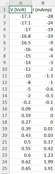
In a laboratory experiment, data of voltage and current has been recorded and the same is attached in an excel file ( Click on this link VI.xlsx ). Read the excel file in the Matlab program and perform the interpolation in the range of -17.3:0.1:0.9. Generate the interactive plot for the interpolated data and store them in a text file.

Key Highlights:

• Graphical solutions are more visual and appealing
• Interpolation of data
• Read excel file
• Write to text file

Deliverables:

• Find missing data and save it in text
• Interpolate the data set
• Save your program and attach the same.
• Save txt file and upload in attachment

AIM

• In this project, the MATLAB code is reading the excel file.
• Execute the interpolation between -17.3:0.1:0.9
• The interpolated data should be generated into an interactive plot and saved in a text file.

INTRODUCTION

The principal applications of interpolation are in mathematics, image scaling, and digital signal processing techniques. Many statistical models can be created using interpolation techniques. Interpolation is a method for integrating new data points between known data points in a range. To fill in gaps in data, smooth out existing data, create forecasts, and more, utilise interpolation. The two types of interpolation in MATLAB are for scattered data points and data points on a grid.

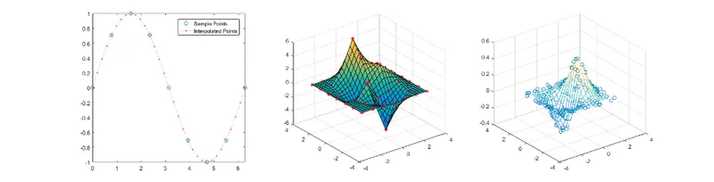
The below attached table is mentioning the interpolation functions

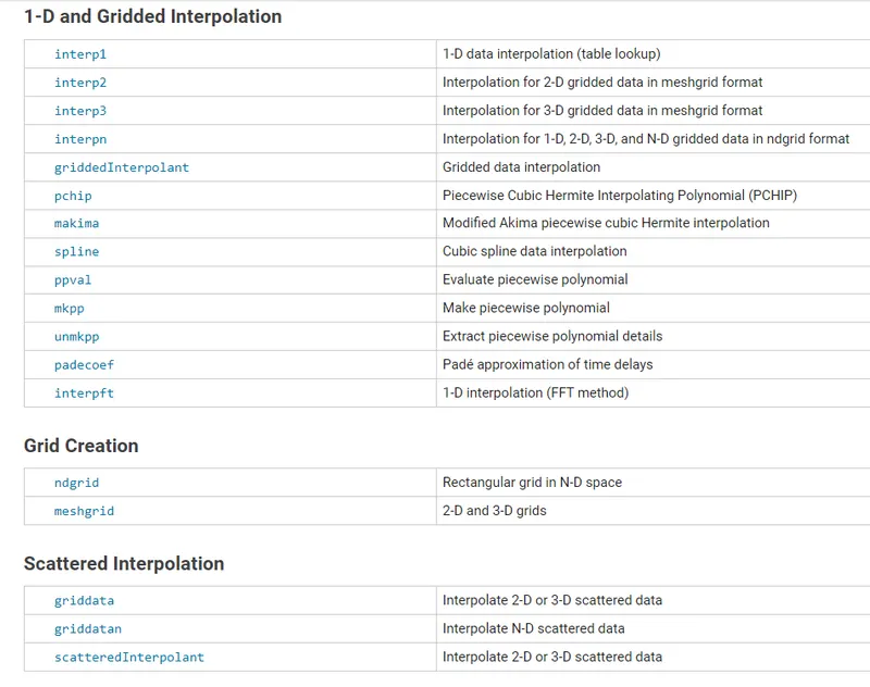
Several interpolation techniques include:

• Using linear interpolation
• interpolation based on closest neighbour or Interpolation that is piecewise constant
• Interpolation using polynomials
• Interpolation using spline
• Interpolation that mimics
• Square Spline Interpolation

MATLAB CODE

xls file

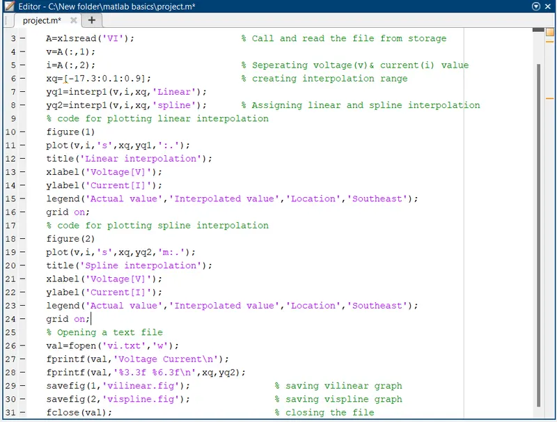
Code

A=xlsread('VI'); % Call and read the file from storage
v=A(:,1);
i=A(:,2); % Seperating voltage(v)& current(i) value
xq=[-17.3:0.1:0.9]; % creating interpolation range
yq1=interp1(v,i,xq,'Linear');
yq2=interp1(v,i,xq,'spline'); % Assigning linear and spline interpolation

% code for plotting linear interpolation
figure(1)
plot(v,i,'s',xq,yq1,':.');
title('Linear interpolation');
xlabel('Voltage[V]');
ylabel('Current[I]');
legend('Actual value','Interpolated value','Location','Southeast');
grid on;

% code for plotting spline interpolation
figure(2)
plot(v,i,'s',xq,yq2,'m:.');
title('Spline interpolation');
xlabel('Voltage[V]');
ylabel('Current[I]');
legend('Actual value','Interpolated value','Location','Southeast');
grid on;

% Opening a text file
val=fopen('vi.txt','w');
fprintf(val,'Voltage Current\n');
fprintf(val,'%3.3f %6.3f\n',xq,yq2);
savefig(1,'vilinear.fig'); % saving vilinear graph
savefig(2,'vispline.fig'); % saving vispline graph
fclose(val); % closing the file

Attachment

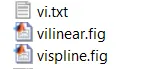
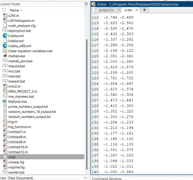
Code Explanation

With the use of the 'clear all' and 'clc' function commands, the memory and storage are cleared.
The 'xlsread ()' function command is used to read the excel file.
Following reading, the current and voltage readings are separated.
by using the instructions "(:,1)" and "(:,2)"
The range of interpolation that must be made is then made in accordance with the question.
By providing the variables v, I and interpolation range, the function "Interp1()" does the linear interpolation. The "interp1()" function, which specifies "spline" as the interpolation method, is used to do spline interpolation similarly.
The charting is completed after the interpolation.
The commands "figure ()" and "plot ()" are used to display the figure and create the plot, respectively.

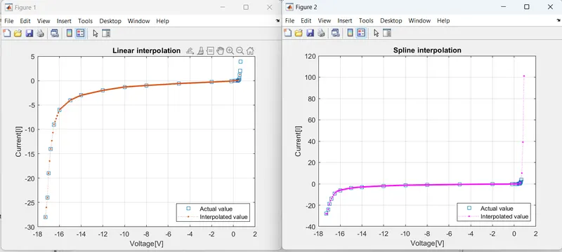
By providing the actual values of voltage v and current I as well as the's' indicated the square form of marker, the linear interpolation is plotted using the figure(1) command and plot command. Additionally, the interpolation of the voltage and current was also depicted in the same figure using the variables xq and yq1 with the indicator ".
The x-axis and y-axis are labelled using the 'xlabel ()' and 'ylabel ()' commands, the plot legend's title is given using the 'Title ()' command, the curves are distinguished using the 'Plot Legend' command, and it is displayed in the bottom right corner by using the 'location' and'southeast' commands.

OUTPUT GRAPH

CONCLUSION

The Matlab software reads the excel file and does interpolation for the range -17.3:0.1:0.9.

The interpolated values are plotted interactively, as well as any missing data are identified and saved in a text file.