Project

Aim:

To study and analyze the BAJA all terrain vehicle (ATV) model using simulink and compare between different models.

Objectives:

1. To prepare a technical report explaining the functions of the subsystems and blocks used for preparing the model

2. To explain in detail all the differences between all the five models provided

3. To understand and comment on the results

Types of Model studied:

1. BAJA ATV model without dashboard (cvt model)

2. BAJA ATV model - data extraction(cvt model_data)

3. BAJA ATV model with Dashboard(cvtmodel_dashboard)

4. BAJA ATV model- Mapped lookup table without dashboard(cvt model_mapped)

5. BAJA ATV model- mapped lookup table with dashboard(cvt model_dashboard_mapped)

Introduction:

CVT: CVTs stands for continuously variable transmission. It is an automatic transmission that can change seamlessly through a continuous range of gear ratio. This contrasts with other transmissions that provide a limited number of gear ratios in fixed steps. The flexibility of a CVT with suitable control may allow the engine to operate at a constant RPM while the vehicle moves at varying speeds.

In its simplest form it can be explained as there are two pulleys when one pulley contracts the othr one expands. This contraction and expansion also result in changing the area of contact of the belt vary accordingly. For example, if the primary pulley is in the contracted position that means more area of belt is in contact with the pulley and on the other hand the secondary pulley is going to be in an expanded position. This results in bigger pulley at one end and smaller at others. which means if the input pulley is bigger and output is smaller, for 1 rotation of input pulley output pulley will rotate more number of turns and a speed increment will be achieved.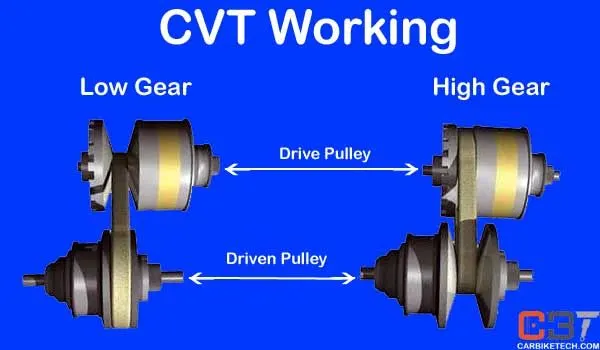

On the other hand, if the input pulley is smaller(expanded) and output pulley is bigger(contracted) speed reduction will be there, as for several rotations of input pulley the output pulley will rotate by single rotation and a speed reduction will be achieved.

The step less nature of its design allows the CVT to work to keep the engine in its optimum power range, increasing efficiency and fuel mileage by delivering an infinite number of smooth transitions from low to high.

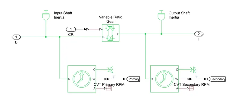
Both the base and the follower(primary and secondary) are given inertia elements to make the model more realistic. Rotational motion sensors are connected to measure the rpm of both sides.

PORTS,

1. B - Base Pulley or Drive Pulley
2. F - Follower Pulley or Driven Pulley
3. r - Variable Transmission Ratio (Input)

The most common type of CVT uses two pulleys connected by a belt or chain. Depending upon the position of variator of the secondary and primary pulley, speed reduction and overdrive take place.

In order to connect engine and CVT a speed reduction is necessary and it is achieved using a gear ratio with a gear ratio of 4.

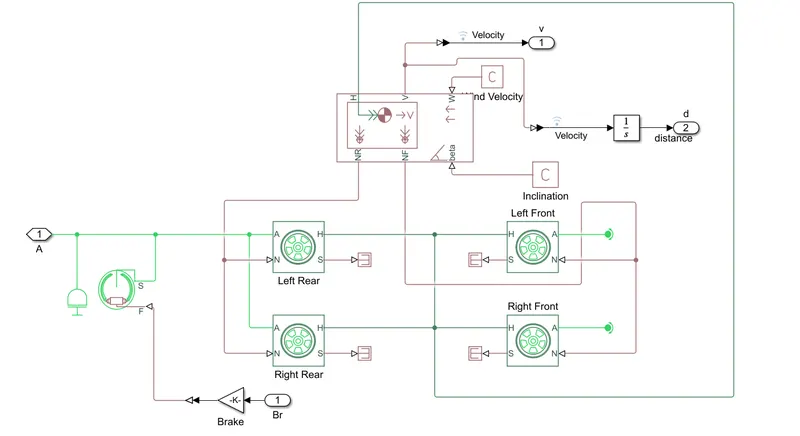
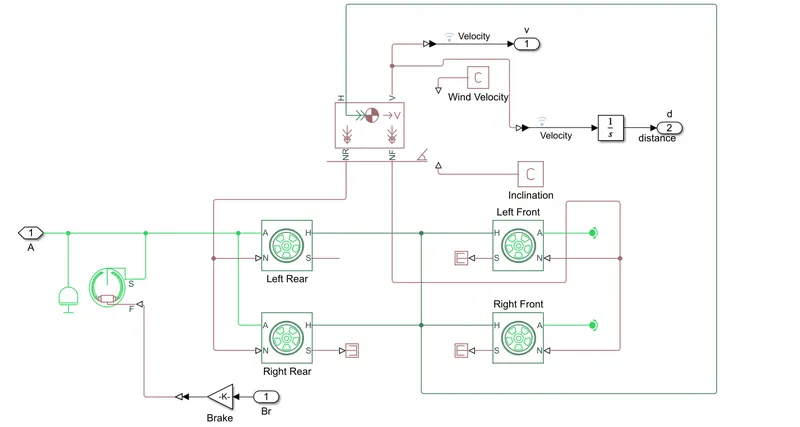
The four wheels are connected accordingly and rpm of the secondary of CVT and brake input is given to the subsystem. The vehicle body is given zero inclination and wind velocity. The velocity is taken to the scope by using an Outport block.

Two-axle vehic le with longitudinal dynamics and motion and adjustable mass,geometry,and drag properties. The vehicle can have the same or a different number of wheels on each axle. For example,two wheels on the front axle and one wheel on the rear axle.The vehicle wheels are assumed identicalin size.The vehicle can also have a centre of gravity (CG) that is at or below the plane of travel.

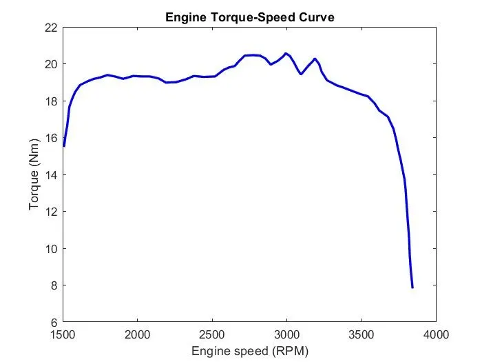
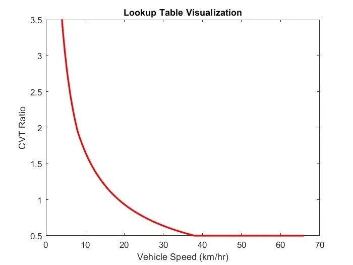
In order to give inputs the speed and torque values are taken from the curve. This curve is represented below.

Lookup Table:
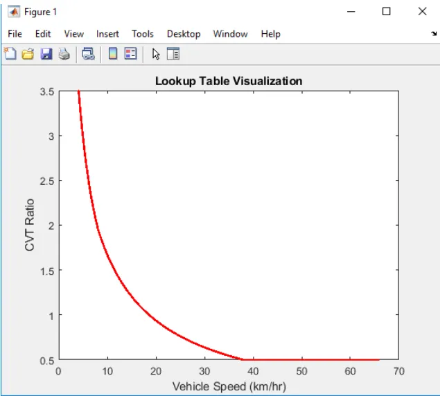
- These are used to map output based in input given. The output data corresponding to input is linked using a data array defined in the lookup table. Lookup table improves accuracy and reduces the t ime. Using Interpolation and Extrapolation Simulink can extract other data.

- The lookup table in this model gives the CVT ratio as output for respective input vehic le speed.In order to calculate the CVT ration,the vehicle speed is fed back to the CVT subsystem,where using the table block it is calculated.

Data instructor is also used to run the simulation for multiple masses.

VEHICLE BODY :-

Two-axle vehicle with longitudinal dynamics and motion and adjustable mass,geometry,and drag properties. The vehicle can have the same or a different number of wheels on each axle. For example,two wheels on the front axle and one wheel on the rear axle. The vehicle wheels are assumed identical in size. The vehicle can also have a centre of gravity (CG) that is at or below the plane of travel.

PORTS,

1. NR - Rear Axle Normal Force (N) ii. NF - Front Axle Normal Force (N) iii. Beta - Road Incline Angle (rad) i V - LongitudinalVelocity (m/s)

2. w - Head Wind Speed (m/s)

3. H - Horizontal Motion

DOUBLE SHOE BRAKE:-

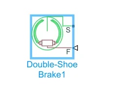
The Double-Shoe Brake block represents a frictional brake with two pivoted rigid shoes that press against a rotating drum to produce a braking action.The rigid shoes sit inside or outside the rotating drum in a diametrically opposed configuration.A positive actuating force causes the rigid shoes to press against the rotating drum.Viscous and contact friction between the drum and the rigid shoe surfaces cause the rotating drum to decelerate.

PORTS:

1. S - Rotational conserving port associated with the rotating drum shaft
2. F - Physical signal input port associated with the appliedactuating force

Tire:

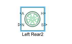
The vehicle body is connected to 4 tires each per axle to move the vehicle according to the power input to the axle.

PORTS:

1. A - Axle
2. H - Mechanical translational port associated with the wheel hub that transmits the thrust generated by the tire to the remainder of the vehicle
3. N - Normal Force
4. S - Tire Slip

The Tire (Magic Formula) block models a tire with longitudinal behavior given by the Magic Formula, an empirical equation based on four f itting coeffic ients. The block can model t ire dynamics under constant or variable pavement condit ions. The longitudinaldirection of the tire is the same as its direction of motion as it rolls on pavement. This block is a structural component based on the Tire road interaction block.To increase the fidelity of the tire model,you can spec ify properties such as tire compliance,inertia,and rolling resistance. However,these properties increase the complexity of the tire model and can slow down simulation.Consider ignoring tire compliance and inertia if simulating the model in real time or if preparing the model for hardware-in-the-loop (HIL) simulation.

Other Blocks used:

1. Solver Conf iguration - To specify the solver parameters before start ing the simulation
2. Signal Builder - To input the Brake,Throttle and CVT Ratio
3. Simulink to PS Converter - To convert the Simulink signal to Simscape environment
4. PS to Simulink Converter - To convert Simscape signal to Simulink environment
5. Mechanical Reference - To make sure all the components are clamped to the ground
6. Rotational free end:The Rotational Free End block represents a mechanical rotational port that rotates freely, without torque.
7. Scope - To display different graphs
8. Display - To view the calculated engine power
9. Inertia - To represent the solid inertia
10. Rotational Motion Sensor - To sense the rotationalmotion from the engine and give output as rpm
11. PS Terminator - Terminator for unconnected physical signal outputs
12. PS Constant - Generate constant physical signal
13. Rotational Free End - For mechanical component (Tire)
14. Custom Measure Gauge - To measure the brake and throttle input
15. Knob - To increase,decrease and vice-versa of throttle and brake inputs
16. Lookup Table - To insert the CVT values from the workspace
17. Step - To increase or decrease an input value for a def ined time interval

Model#1: Simulation of BAJA ATV model with CVT:

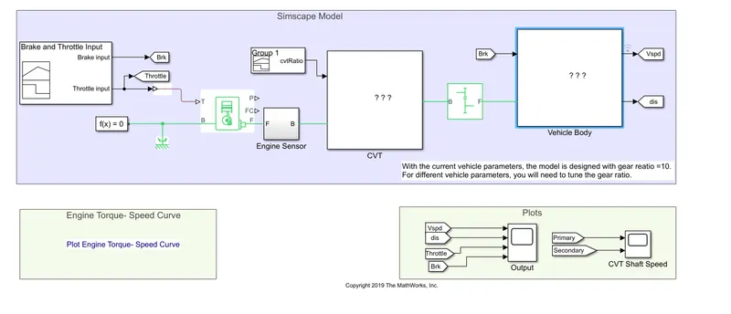
Steps:

1. The throttle signal is generated by signal builder block and inputted to generic engine.
2. The torque and speed vector are inputted f rom the matlab workspace
3. The engine will generate the output rpm which can be taken from the crankshaft outpu This speed will be given to the Ideal Rotational Motion Sensor to sense the output rpm.
4. The same output speed will be given to a simple gear mechanism to reduce the speed where the Gear Ratio is '4'.
5. Then the output speed from the gear reducer will be given to the Variable Ratio Transmission block (CVT).
6. The CVT ratio is provided to the Variable Ratio Transmission (CVT) block through Signal Builder.
7. The speed is controlled by the variable CVT ratios and the controlled output speed is inputted to the vehicle axle.
8. brake signal is generated by the signal builder and inputted to the vehicle body (Double Shoe Brake) for applying the brake to axle
9. The power from the CVT is inputted to the axle and the vehicle accelerates according to the speed.
10. Then the Velocity is taken as output from the vehicle body for f urther analysis.

Input signals:

Throttle input signal:

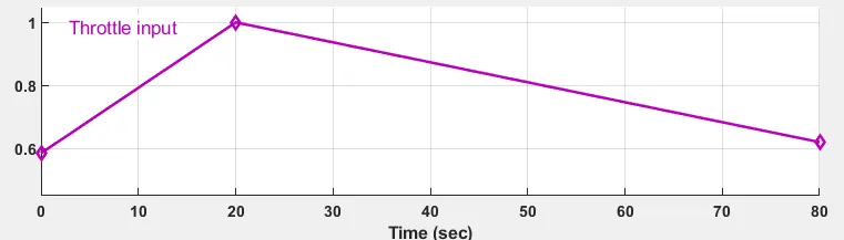
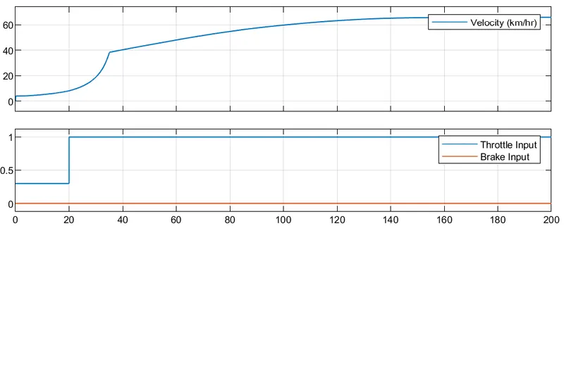
Throttle starts at 0.3 and then it steps t o1 at the 20th second

Brake input signal:

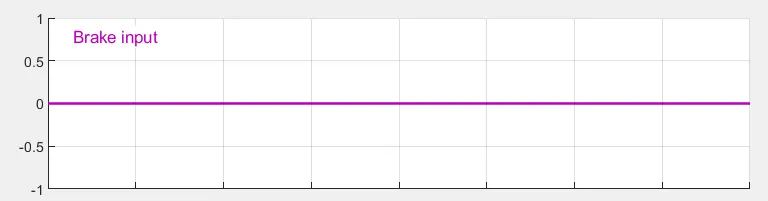
The brake input remains zero through the whole simulation There are two inputs provided using signal builder one is the break input given a 0 value other is a throttle input which has a value of 0.25 for 20 s and is increased to land remains same for total80s. Both these are fed to the a eneric engine.

• The throttle which is input is fed to T import This establishes a relation between speed and torque. Connections F and B are mechanical rotational conserving ports associated with the engine crankshaft and engine block, respectively. Connections P and FC are physical signal output ports through which engine power and fuel consumpt ion rate found out and transmitted to further systems. The port F is connected to a sensor which finds the angular velocity and displacement of the crankshaft.
• In the model in order to restrict a high rpm from the engine gear is used before feeding the rpm values to the CVT
• The engine speed-torque characteristics are also represented above CVT

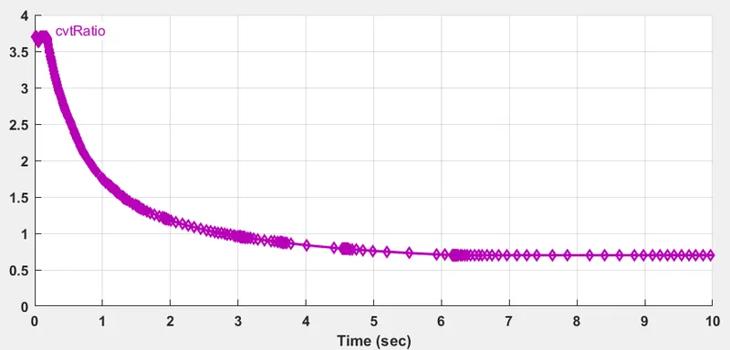
There are two pulleys a primary which is the driver and secondary which is driven

These have an input and output shaft inertia respectively

The variable-ratio gear block provides the different gear ratios ( represents multiple gears of CVT)

The gear ratio input is fed to the r port of the above block

The angular velocity of the two pulleys is tracked using ideal rotational sensors.

The input to the CVT is defined using a signal builder block

Result and observations for case1

a. Engine torque vs speed

The value of starting torque is very high which is neede for pick up

b. vehicle speed curve

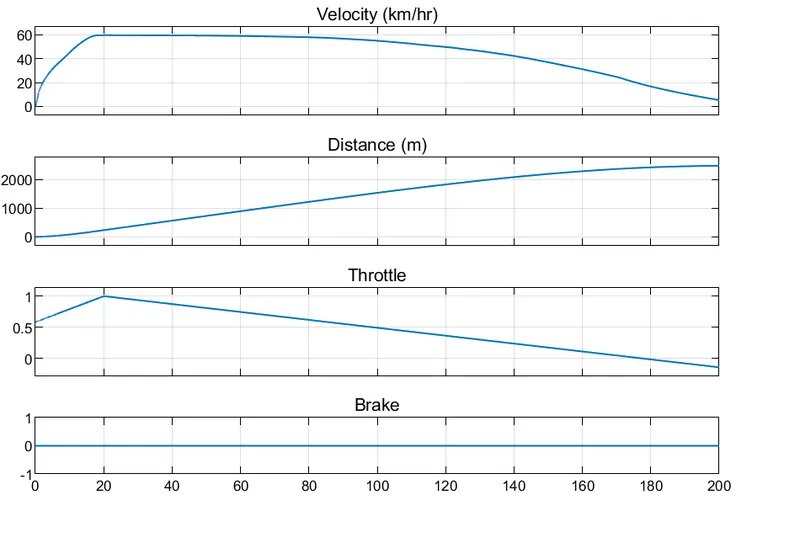
The throttle input changes from 0.3 to 1 after 20 s. That can be seen in the graph that as a change in throttle occurs similar to wot and the lack of a brake the vehicle speed keeps on increasing till it attains a top speed

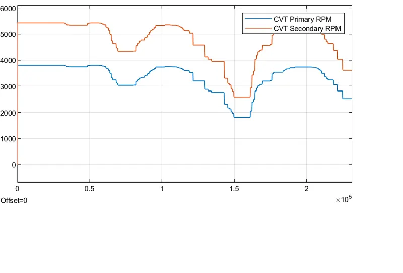
3. CVT shaft speed:

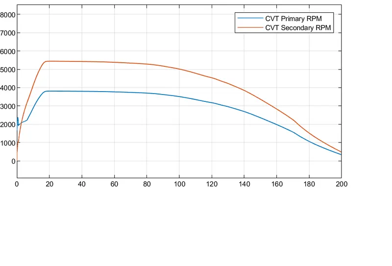
The effect on CVT can be studied by dividing the above into 3intervals.

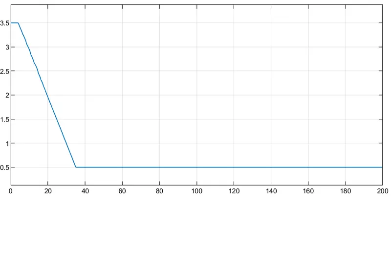
1st- 0 to 20 s-During the initial period the CVT ratio is high.This can be visualized as synonymous to gear ratio. By def inition,in terms of rpm,it is the speed of the input shaft to speed to the output shaft in this context. During this period the driver will have a small diameter and the driven will have a larger diameter to facilitate the demand for higher torque. CVT ratio: 0-10 s ,> 2 whereas > 30s,0.5

2nd-When there is an increase in throttle value,the speed of the vehicle increases. As this happens the driver starts to increase its diameter thereby a decrease in gear ratio to provide more rpm at driven.

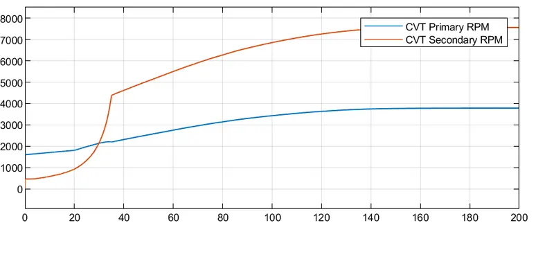
3rd-When there is an increase in the speed of the vehicle it can be seen that there is an increase in rpm of driven( secondary) compared to that of the primary. This means that the f irst pulley will have a larger diameter for a higher rpm and for one rotation of a larger pulley there will be more rotation of driven.CVT ratio keeps on decreasing

Model#2: Simulation of BAJA ATV model with CVT and dashboard:

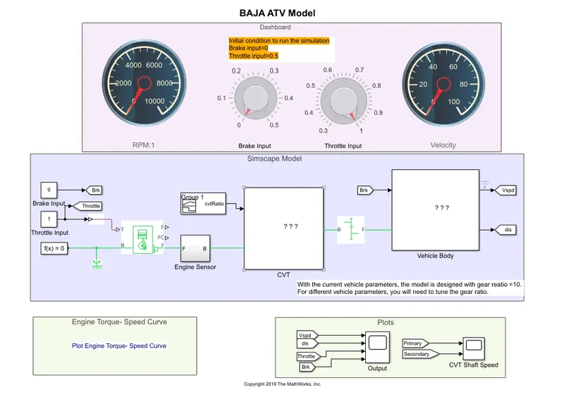
• In the first case the inputs throttle and brake was given as signal builder. But here there are knobs to control the input variables and can be controlled real-time.
• The input knob for throttle starts to 0.3 whereas brake knob is set at 0. The speed is increased in real-time and the brake as wel

Results and observations for case 2:

a. engine torque vs speed

B. vehicle speed curve

The brake input is not changed for the first three seconds whereas the input value of the throttle is changed gradually and at 0.7 at t=l.5. For this period of time,the speed of the vehicle keeps on increasing. After 1.5 sec the brake input is changed f rom 0 gradually which creates a decrease in speed.

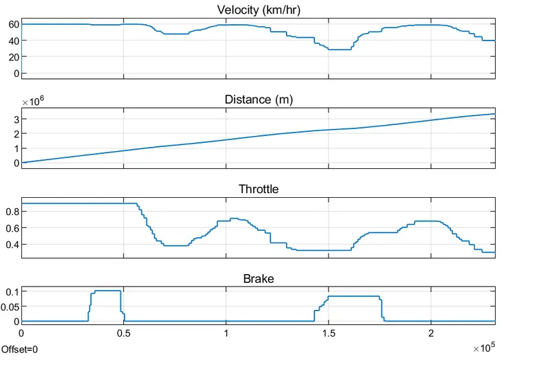
and the result from cvt from the given input from the various input on the dashboard which you might see the result, from the above input you could understand the input given by us and the brake and throttle has increased and decreased.

When there is an increase in throttle command there is an increase in the speed of the vehicle. This leads to a decrease in CVT ratio compared to start where more torque is needed but when there is braking forex at t=3, CVT-0.48 compared tp t=1 ,CVT-0.47.

Model#3: Simulation of BAJA ATV model with a lookup table the difference of feedback.

A lookup table is an array of data that maps input values to output values. This is done so as to approximate a mathematical function.

When a set of input values are known a lookup yield an output value corresponding to each input from a table of values. If the lookup table does not explicit ly define the input values, Simulink helps by estimating an output value using interpolation,extrapolation,or rounding. Interpolation is the process for estimating values that lie between known data points. Extrapolation is the process for estimating values that lie beyond the range of known data points. Rounding is a process for approximating a value by altering its digits according to a known rule.

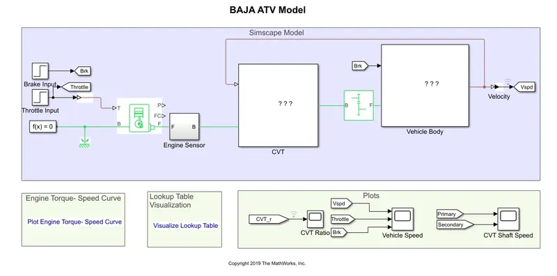
when compared to case 1 and case 2 there exists a difference. The input to CVT is a lookup table which says for a particular CVT ratio what is the speed delivered.

Apart from this the output speed is also tracked as fed to the primary pulley of CVT, thereby acting as feedback for effective reference tracking.

Result and observations for case 3

a. Engine Torque vs speed

b. CVT ratio

c. vehicle speed

d. shat speed

When we compare the above plot, the ratio varies f rom 2.3 - l.8 within timespan of 80 sec which is same as the previous BAJA ATV Models. And from 32 sec it's constant ratio of 'l.8' compared to 35 sec in the first model. A lso the reduction from 2.3 ratio to 1.8 is not perfect ly linear as in the first model.

model#4: Simulation of BAJA ATV model with CVT and dashboard.

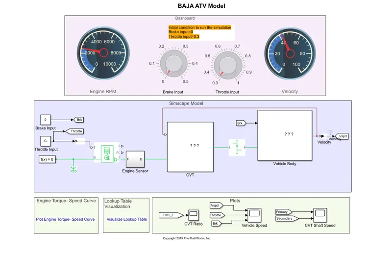
With help of a knob,it is possible to control the throttle and brake inputs.

A lookup table is used to establish a relationship between vehicle speed and CVT.

The initial input value for the throttle is 0.3 but for the brake is 0. Results and observations for case 4

a. Engine torque vs speed:

b. CVT ratio:

c. vehicle speed curve

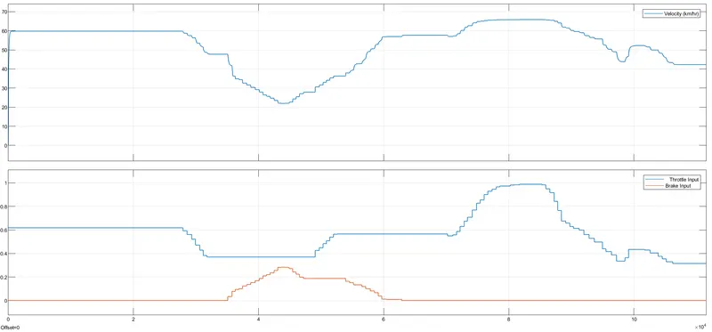
d. cvt shaft speed:

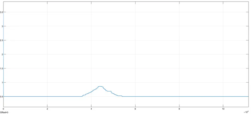
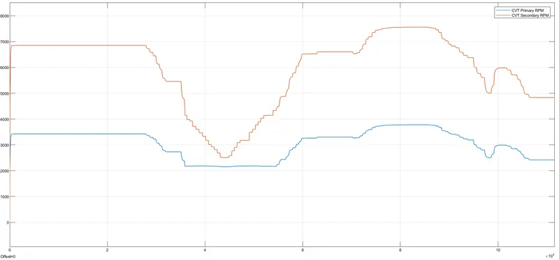When throttle value increases speed increases which is met by an increase in secondary rpm ( rpm of the driven shaft) and during uniform speed,the CVT ratio doesn't change which can be seen via secondary and primary rpm remains constant during these period.

Learning outcome:

Understanding the operat ion of a CVT drive system. Lookup table makes output curves If the lookup table does not explicit ly define the input values, Simulink helps by estimating an output value using interpolation,extrapolation,or rounding giving better quality results To achieve the desired output it is always good to use feedback . As a throttle input increases there happens an increase in speed but the CVT ratio falls when there is an increase in brake input the speed falls but there will be an increase in CVT ratio.