Week 4.1 - Genetic Algorithm

Disclaimer:

explaining about genetic algorithm(ga) and its syntax are in youtube video--https://youtu.be/OQpnw9upnlk

I have code main script one time only. Here im not going to code same script again and again (for my time convinient)

i would code important scripts only

if small changes in code, i particularly code that only,

but share full coding through photocopy

Report:

Initially it was difficult to understand genetic algorithm(ga).

So first i started to finish stalagmite function, simultaneously learning about ga.

I have explored lot of websites and youtube videos to understand optimization.

some useful sites are following

1. nptel source on optimization

2. apmonitor.com

3. mathwork...

4. yarpiz about ga

error:

The error i faced and confusion about setting boudaries at particular position.

optimized value changes every time(not an error but struggle to solve)

getting optimized value beyond graphical area(it take lot of time to find)

------Stalagmite function--------

% stalagmite function looks
% by the formula

function [funv] = stalagmite(input_vector)
x = input_vector(1);
y = input_vector(2);
funv1 = sin(((5.1*pi)*x)+0.5).^6;
funv2 = sin(((5.1*pi)*y)+0.5).^6;
funv3 = exp((-4*log(2))*(x-0.0667).^2/0.64);
funv4 = exp((-4*log(2))*(y-0.0667).^2/0.64);
funv = funv1*funv2*funv3*funv4;
end

so here main script

close all;
clear all;
clc;

% defining our search space
x = linspace(0,0.6,150);
y = linspace(0,0.6,150);

%creating a 2d mesh;
[xx yy]=meshgrid(x,y);

%evaluating the stalagmite function
for i=1:length(xx)
  for j=1:length(yy)
     input_vector(1) = xx(i,j);
     input_vector(2) = yy(i,j);
     f(i,j) = stalagmite(input_vector);
   end
end



%plot
surc(xx,yy,f)
xlabel('x_axis')
ylabel('y_axis')
shading interp


%optimization
[inputs,fval]=ga(@stalagmite,2)

So, when you run it, you get a 3d stalagmite function plot and you get random optimized value

1. inputs

2. fval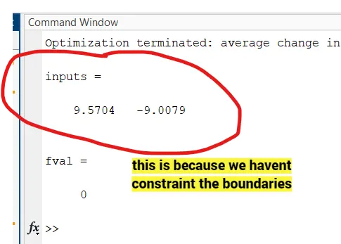

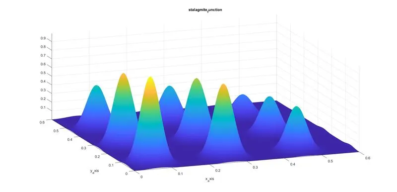
and save it in the name of 'stalagmite.m'

challenge #1

Finding the global maxima

when i explore in online "how to find maxima using ga command?"

I have found the solution in mathwork q&a page:

so what actually found is inverting the function makes the minima into maxima

Inverting the function is nothing but just assinging the negative value for the function

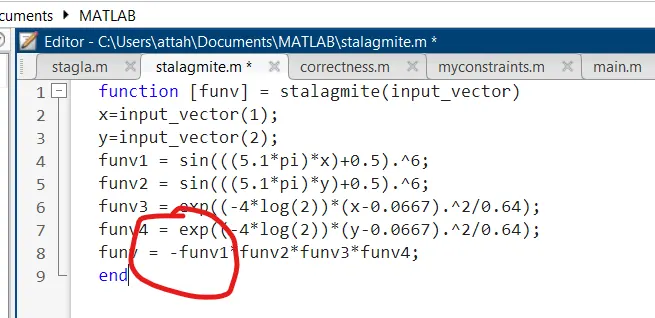
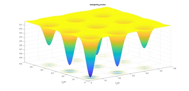
anyhow the 'ga' command going to find the minimum value

So when the function inverse, and you find the minimum then it is maxima.

Manual indicating maxima give below

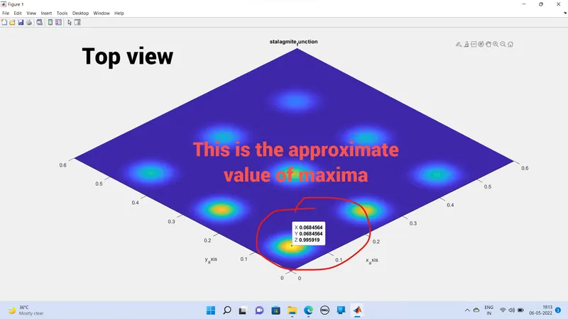
To find maxima using 'ga' command

1st we have set boundaries

lower bound and upper bound

note--If you aren't set boundaries then there would lot of optimal solution for every run.

%boundaries
% to get a single value
lb = [0 0]
ub = [0.2 0.2]

[inputs,fval]=ga(@stalagmite,2,[],[],[],[],lb,ub)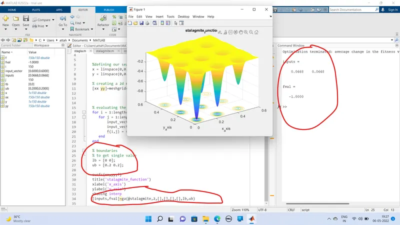

compare with manual value it is almost equal.

so here fval is negative one(-1), because we have assigned the function in negative.

if you want the original maxima value then multiply with negative you get positive one.

so even you run it several times you get the same value

to check

for i=1:50
[inputs,fval]=ga(@stalagmite,2,[],[],[],[],lb,ub)
end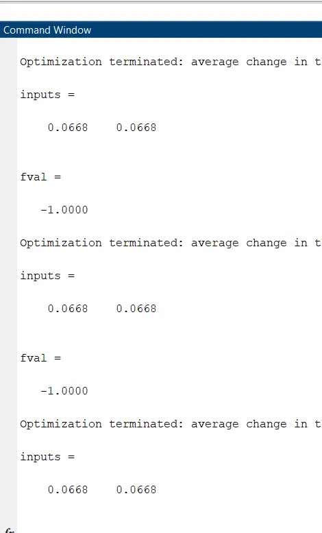

so the above img shows the samevalue for every iteration

finally showing the plot for fmaxima and no of iteration

% until here getting stalagmite function
%i dont want to code it again


% boundaries
lb = [0 0];
ub = [0.6 0.6];

% here i take 100 iteration
for i=1:100
[inputs,fval]=ga(@stalagmite,2,[],[],[],[],lb,ub);
xmax(i) = inputs(1);
ymax(i) = inputs(2);
fmax(i) = fval;
end

figure(1)
subplot(2,1,1)
hold on
plot3(xmax,ymax,fmax,'o','markersize',5,'markerfacecolor','r');
surfc(xx,yy,f)
axis([0 0.6 0 0.6])
title('stalagmit_function')
xlabel('x_axis')
ylabel('y_axis')
shading interp
subplot(2,1,2)
title('iter_bound')
plot(fmax)
xlabel('iteration')
ylabel('fmax')

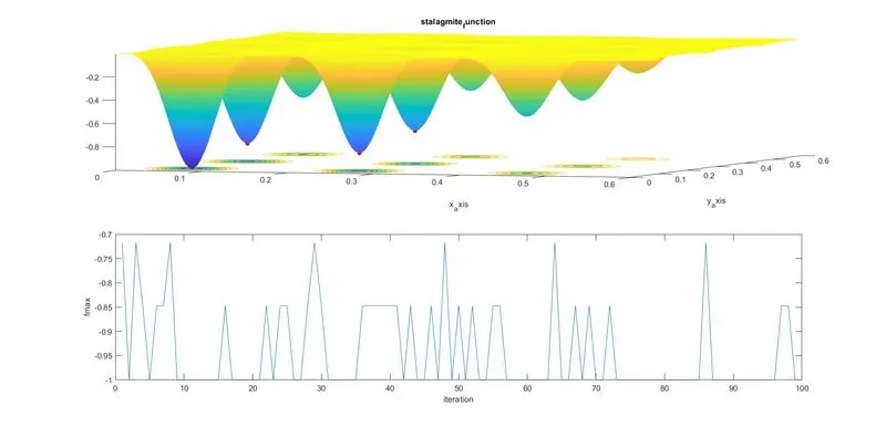
this is for 100 iteration.

and you can see the markerpoint at the edge of the stalagmite peak where the maxima present

explanation and procedure i have done could see in this video---https://youtu.be/OQpnw9upnlk