Project 2 - Rankine cycle Simulator

Rankine cycle simulator

The challenge is to find

• the state points of the Rankine cycle
• to plot the T-S and H-S graph using these state points
• and also to find other parameters

About Rankine Cycle:

The Rankine cycle or Rankine Vapour Cycle is the process widely used by power plants such as coal-fired power plants or nuckear reactors. In this mechanism, a fuel s used to produce heat within a boiler, converting water into steam which then expands through a turbine producing useful work.

1. Process and working:
2. Process 1-2: Isentropic Expansion in the turbine.
3. Process 2-3: Constant pressure Heat rejection in condenser
4. Process 3-4: Isentropic compression in the pump
5. Process 4-1: Constant pressure heat addition in the boiler.

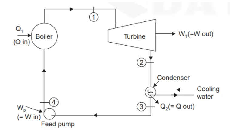
In process 1-2 , The dry saturated vapour expands through a turbine, generating power. This decreases the temperature and pressure of the vapour, and some condensation may occur.

In process 2-3, The vapour liquid mixture leaving the turbine is condensed at low pressure, usually in a surface condenser using cooling water. In well designed and maintained condensers, the pressure of the vapour is weel below atmospheric pressure, approaching the saturation pressure of the operating fluid at the cooling water temperature.

In process 3-4, The pressure of the condensate is raised in the feed pump. Because of the low specific volume of liquids, the pump work is relatively small and often neglected in thermodynamic calculations.

In pocess 4-1, High pressure liquid enters the boiler from the feed pump and is heated to the saturation temperature (on the saturation curve). Further addition of energy causes evaporation of the liquid until it is fully converted to saturated steam or superheated.

Now start with finding state points from XSteam file

• Usually start with clear all, close all and clc command to clear and delete and close the previous variable, data or window which stores the old datas
• Using disp command to show the four process in the command window
• Then to get the value of unknown, I have use the input command to get value from user
• To access the function(XSteam) output we have to give the input required

Just like solving free hand Rankine cycle problem we need to find some initial values and some are given.

So to find through steam table, here we find by xsteam function

clear all
close all
clc

disp('Rankine cycle Simulator');
disp('1-2 is Isentropic expansion in turbine');
disp('2-3 is isobaric heat rejection in condensor');
disp('3-4 is isentropic compression in pump');
disp('4-1 is isobaric heat addition in boiler');

%Inputs
p1 = input(' enter turbine inlet pressure in bar: ');
t1 = input('enter turbine inlet temperature in degree celcius: ');
p2 = input(' enter condensor pressure in bar: ');

%Inlet of the Turbine
% state 1
s1 = XSteam('s_pT',p1,t1);    % extracting enthalpy at state
h1 = XSteam('h_pT',p1,t1);    % similarly

% Inlet of the condenser
% state 2
s2 = s1;
t2 = XSteam('Tsat_p',p2);
sf2=XSteam('sL_p',p2);
sg2 = XSteam('sV_p',p2);
hf2 = XSteam('hL_p',p2);
hg2 =XSteam('hV_p',p2);
x2 = ((s2-sf2)/(sg2-sf2)); %dryness fraction factor
h2 = hf2+(x2*(hg2-hf2));

% Exit of the condenser
% state 3
p3 = p2;         %costant pressure heat rejection
t3 = t2;
s3 = XSteam('sL_T',t3);
h3 = XSteam('hL_p',p3,s3);

%inlet to the boiler
% state 4
p4 = p1;
s4 = s3;
h4 =XSteam('h_ps',p4,s4);
cp4 =XSteam('CpL_p',p3);
cv4 = XSteam('CvL_p',p3);
gamma = (cp4/cv4);
t4 = XSteam('T_ps',p4,s4);

After we have found the state points, lets find other important parameters

To find that parameters we use formulas used in thermodynamic

% Other parameters of Rankine cycle

% other states on curve
tp = XSteam('TSat_p',p4);
tq = tp;
sq = XSteam('sV_T',tq);
sp = XSteam('sL_T',tp);

% calculation
tq = tp;

%workdone by turbine
wt = h1 - h2;

%work done by pump
wp = h4 - h3;

% back work ratio
b_w_r = wp/wt;

%back work ratio in percetage
B_w_r = b_w_r*100;

%net work done
w_net = wt - wp;

%heat injected in boiler
q_in = h1 - h4;

%heat rejected in condensor
q_out = h2 - h3;

%thermal efficiency
n = w_net/q_in;
np = n*100;

Here Back work Ratio is new term

lets explain about that:

The back work ratio is just the fraction or percentage of the work that the turbine produces that is consumed by the pump. The lower the back work ratio, the better the performance of the power plant.

Back work ratio = pump work/turbine work

In percent = Back work ratio * 100

Then plot the state points and saturation curve:

First we code the program for Temperature vs entropy

%plot for temperature vs entropy
figure(1)

%plot for liquid and vapour saturation curves
t = linspace(0,550,600);

for i = 1:length(t)
    s_l(i) = XSteam('sL_T',t(i));
end

for i = 1:length(t)
    s_v(i) = XSteam('sV_T',t(i));
end

plot(s_l,t,'r','linewidth',1)
hold on 
plot(s_v,t,'r','linewidth',1)


%%plot of work done by turbine
plot([s1,s2],[t1,t2],'color','k','linewidth',2) 

%plot for heat rejected in condensor
plot([s2,s3],[t2,t3],'color','k','linewidth',2)

%plot for workdone by pump
plot([s3,s4],[t3,t4],'color','k','linewidth',2)

%plot for heat injected by boiler
plot([s4,sp],[t4,tp],'color','k','linewidth',2)

plot([sp,sq],[tp,tq],'color','k','linewidth',2)

plot([sq,s1],[tq,t1],'color','k','linewidth',2)

%plot decoration
title('T-S diagram of Rankine cycle')
xlabel('entropy(KJ/K)')
ylabel('Temperature(k)')
grid on

%Indicate states with numbers
text(s1,t1,'1','color','b');
text(s2,t2,'2','color','b');
text(s3,t3,'3','color','b');
text(s4,t4,'4','color','b');

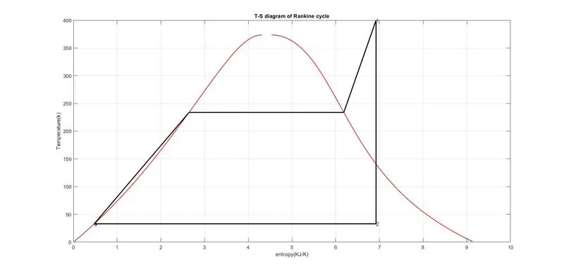
we plot the saturation line in red color and Rakine cycle path in black color by asked in challenges:

Now Enthalpy vs Entropy

%plot for enthalpy vs entropy
figure(2)

plot([s1,s2],[h1,h2],'color','k','linewidth',2)
hold on
plot([s2,s3],[h2,h3],'color','k','linewidth',2)

plot([s3,s4],[h3,h4],'color','k','linewidth',2)

plot([s4,s1],[h4,h1],'color','k','linewidth',2)


%plot for liquid and vapour saturation curve
t = linspace(0,550,600);
for j = 1:length(t)
    h_l(j) = XSteam('hL_T',t(j));
end

for j=1:length(t)
    h_v(j) = XSteam('hV_T',t(j));
end

plot(s_l,h_l,'linewidth',1,'color','r')

plot(s_v,h_v,'linewidth',1,'color','r')

%decoration of graph
grid on 
title('H-S diagram for Rankine cycle')
xlabel('entropy (KJ/K)')
ylabel('enthalpy(KJ/Kg)')


%Indicate sates with numbers
text(s1,h1,'1','color','b');
text(s2,h2,'2','color','b');
text(s3,h3,'3','color','b');
text(s4,h4,'4','color','b');

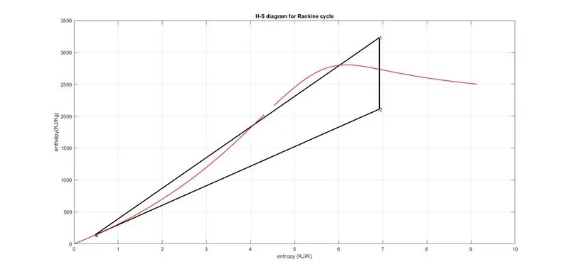
same as before saturation line in red color and curve path in black color

Finally visuallizing is the challenging thing compare with other things.

so I would like to explain something about fprintf

fprintf command used for Formatting the output data

fprintf(fileID,formatspec,A1...An)

Actually it need time to learn and it has somecode format to learn initially

so my reference here---https://www.youtube.com/watch?time_continue=4&v=tS4fmMPE7kI&feature=emb_logo

% results output

fprintf('%s %44s\n','At State point 1: ','At state point 3: ')
fprintf('%s %.3f %s %38s %.3f %s\n','P1 is : ',p1,'Bar','P3 is : ',p3,'Bar')
fprintf('%s %.3f %s %29s %.3f %s\n','T1 is : ',t1,'Deg Celcius','T3 is : ',t3,'Deg Celcius')
fprintf('%s %.3f %s %34s %.3f %s\n','H1 is : ',h1,'KJ/Kg','H3 is : ',h3,'KJ/Kg')
fprintf('%s %.3f %s %36s %.3f %s\n\n','S1 is : ',s1,'KJ/KgK','S3 is : ',s3,'KJ/KgK')

fprintf('%s %44s\n','At State point 2: ','At state point 4: ')
fprintf('%s %.3f %s %39s %.3f %s\n','P2 is : ',p2,'Bar','P4 is : ',p4,'Bar')
fprintf('%s %.3f %s %30s %.3f %s\n','T2 is : ',t2,'Deg Celcius','T4 is : ',t4,'Deg Celcius')
fprintf('%s %.3f %s %34s %.3f %s\n','H2 is : ',h2,'KJ/Kg','H4 is : ',h4,'KJ/Kg')
fprintf('%s %.3f %s %36s %.3f %s\n\n','S2 is : ',s2,'KJ/Kgk','S4 is : ',s4,'KJ/KgK')

fprintf('Other calculations\n')
fprintf('Turbine Work is : %.3f KJ/Kg\n',wt);
fprintf('Pump work is : %.3f KJ/Kg\n',wp);
fprintf('Efficiency is : %.3f percent\n',np);
fprintf('Heat input is : %.3f KJ/kg\n',q_in);
fprintf('Heat rejected is : %.3f KJ/Kg\n',q_out);
fprintf('Wnet is : %.3f KJ/Kg\n',w_net);
fprintf('Back work ratio is : %.5f \n',b_w_r);

So another challenge is to visuallize as same as like given in the question

here is the picture down below shows exact image of given:

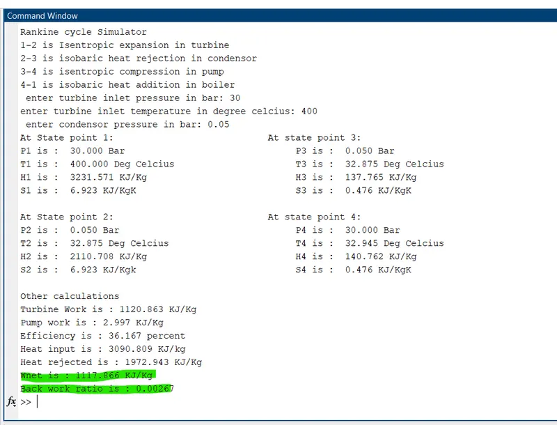
So, The Net work output is 1117.866 (KJ/Kg)

and the Back work ratio is 0.00267 (no unit)

As before said, The lower the back work ratio, the better the performance of the power plant.

Error I have faced:

some typing mistakes and some usual paranthesis error

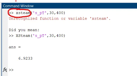
call xsteam function with small letters instead XSteam is correct

Initially the program has struck without any changes

then i call the function separately in command window and I have understand