Week 3 - Solving second order ODEs

https://youtu.be/cHOvnPOt_UQ

REPORT:

Solving second order ode using "ode45" command is really useful for other ode problems,

Initially it is bit difficult to understand and challenging.

Using marker command is new thing, and i use it as a pendulum ball.

The output from ode45 funtion is two column(what i get 1.displacement 2.angular velocity)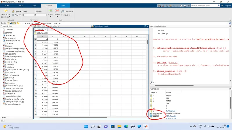

where t is usual independent value i used here

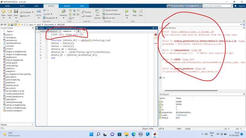
I have made some mistakes during coding

1. using close all;clear all; clc; command in function folder which is error
2. some parenthesis mistakes
3. and some typing mistakes which computer couldnt recongnize the variables
4. 

% solving second order ode of simple pendulum motion
% program start with function folder

function [dtheta_dt] = odefun(t,theta,b,g,l,m)
theta1 = theta(1);
theta2 = theta(2);
dtheta1_dt = theta2;
dtheta2_dt = -(b/m)*theta2-(g/l)*sind(theta1);
dtheta_dt = [dtheta1_dt;dtheta2_dt];
end
% save this folder in the name of odefun.m


% open other folder (simple_pendulum.m)

clear all;
close all;
clc;

% assigning the value
b = 0.05;
g = 9.81;
l = 1;
m = 1;

% initial condition
theta_0 = [0;3];    % where 3 is for initial angular velocity

% Time points
t_span = linspace(0,100,500);

% SOLVE ODE
programme = @(t,theta) odefun(t,theta,b,g,l,m);

[t,results] = ode45(programme,t_span,theta_0);

% graph
figure(1)
plot(t,results(:,1))
hold on
plot(t,results(:,2))
ylabel('angular velocity and distance')
xlabel('time')
legend('distance','angular velocity')


% animation
x0 =0; y0= 0;
ct=1
for i = 1:length(t)
x1 = l*sind(results(i,1));
y1 = -1*cosd(results(i,1));

figure(2)
plot([-1 1],[0 0],'linewidth',6,'color','g');
axis([-2 2 -2 2]);
line([x0 x1],[y0 y1],'linewidth',4,'color','b');
hold on;
plot(x1,y1,'o','markersize',20,'markerfacecolor','r');
hold off
M(ct)=getframe(gcf)
ct = ct +1;
end

% saving as movie
movie(M)
videofile = VideoWriter('simple_pendulum','uncompressed AVI');
open(videofile);
writeVideo(videofile,M);
close(videofile);

% ok, run it

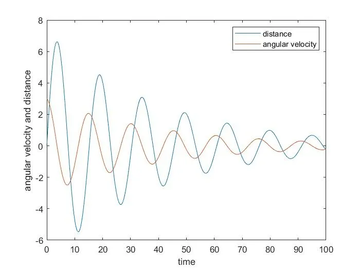animation https://youtu.be/cHOvnPOt_UQ