Project

AIM:

To study the model of BAJA All terrain vehicle(ATV) and to analyze the simulation results.

OBJECTIVE:

To Create a technical report on BAJA All Terrain Vehicle.

THEORY:

ATVs are off-road vehicles that are commonly used for recreation. It is permissible in most places for older youngsters and teens to ride without a driver's licence. However, the delights come with significant safety concerns. ATVs, especially at high speeds, can be unstable and difficult to handle. Rollovers and collisions occur often, and some are fatal. ATV-related injuries are very common and might result in a trip to the emergency department. As a result, the American Academy of Pediatrics (AAP) advises children and teenagers aged 16 and under not to drive or ride ATVs.

An all-terrain vehicle (ATV) is a motorised off-highway vehicle with a seat designed to be straddled by the operator and handlebars for steering control that travels on four low-pressure or non-pneumatic tyres. ATVs are separated into two types based on the manufacturer's designation. The manufacturer designed Type I ATVs to be operated by a single person with no passengers. The manufacturer designed Type II ATVs to be used by an operator and a passenger, with a defined seating place behind the operator. Riders must also take into account the varying ATV sizes.

The Society of Automotive Engineers International hosts the Baja SAE Collegiate Design Series competition (SAE International). Small off-road cars are designed and built by teams of students from universities all over the world. The engines in all of the vehicles are identical. The engine is a single-cylinder Briggs & Stratton Model 19 Vanguard engine with a displacement of 305cc and a power output of roughly 10 horsepower (7.5 kW) as of 2018.

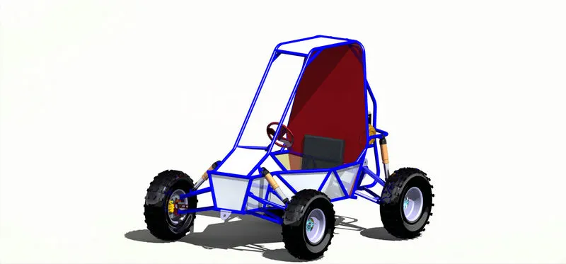
Here we are analyzing Baja ATV model with dashboard and without dashboard using Simulink.

MODEL OF BAJA ATV WITHOUT DASHBOARD:

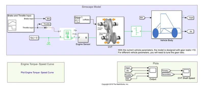
Now we are breaking the model to analyze each subsystem used to model this ATV.

Vehicle Body:

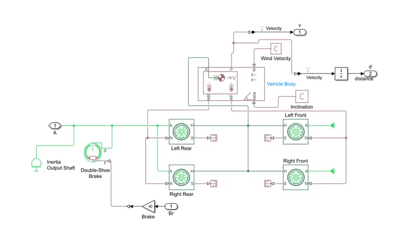
The vehicle body constitute of 4 tyres and braking system and a vehicle body block with its model parameters.

Tyre:

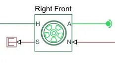
The tyre Magic Formula characterises the longitudinal behaviour of a highway tyre. Tire-Road Interaction (Magic Formula) and Simscape Foundation Library Wheel and Axle blocks are used to construct the block. The impacts of tyre inertia, stiffness, and damping can be incorporated as an option. The mechanical rotational conserving port for the wheel axle is Connection A. Connection H is the wheel hub's mechanical translational conserving port, via which the tire's push is applied to the vehicle. The normal force acting on the tyre is applied by Connection N, which is a physical signal input port. When a force acts downward, it is termed positive. The tyre slip is reported by Connection S, which is a physical signal output port.

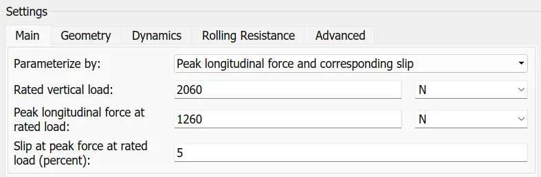
Here the A port is connected to a Rotational free end which means it is allowed to rotate freely and S port is attached to a PS terminator which terminates the physical signal. In case of rear wheels the A port is connected to the input braking signal.

Vehicle Body:

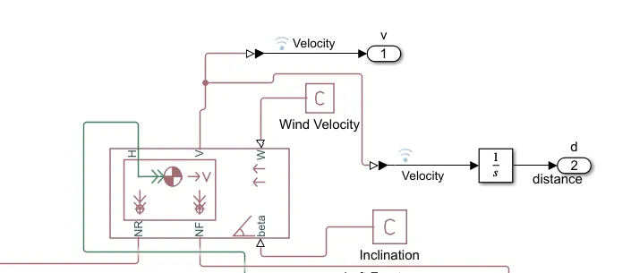
The block represents the longitudinal motion of a two-axle vehicle body. Due to acceleration and road profile, the block accounts for body mass, aerodynamic drag, road gradient, and weight distribution between axles. Each axle can have the same number of wheels or a different number of wheels. Pitch and suspension dynamics, as well as additional changeable mass and inertia, are optional. In relation to the ground, the vehicle does not move vertically. Connection H is the horizontal motion of the vehicle's body's mechanical translational conserving port. This port should be connected to the traction motion created by the tyres. The physical signal output ports V, NF, and NR are for vehicle velocity and front and rear normal wheel forces, respectively. When wheel forces act downward, they are called positive. Physical signal input ports W and beta correspond to headwind speed and road inclination angle, respectively.

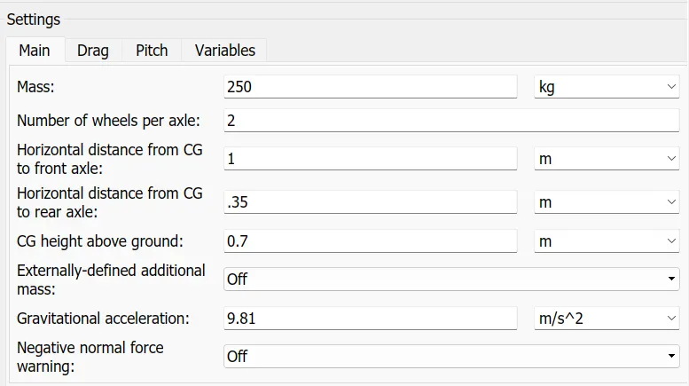
Here NF and NR are connected to the rear and front wheels, beta is connected to a PS constant of value 0 inclination and W is connected to a PS constant of value 0 as wind velocity. H is connection to the hub and V gives the vehicle velocity which is used to find out the distance covered.

Braking system:

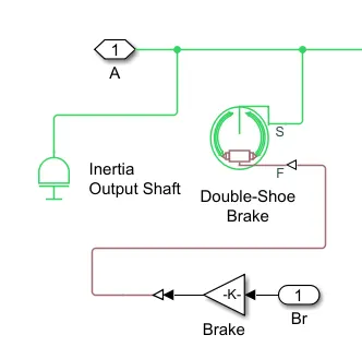
The mechanical output from the simple gear is connected to the Double shoe brake along with the output shaft inertia of value 1e-1 kgm2. The double shoe brake represents a brake with two pivoted stiff shoes mounted symmetrically inside or outside a drum and controlled by a single actuator. The shoes exert a friction torque on a shaft linked to the drum as a result of the actuator force. The drum shaft is connected to Connection S, which is a conserving rotational terminal. Connection F is a physical signal port that represents the actuator's force input. Positive force produces friction torque, which prevents the shaft from rotating. The braking signal is connected to the F port of the double shoe brake with a gain value of 1000.

Simple Gear:

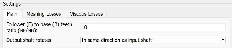
A fixed-ratio gear or gear box is represented by the simple gear. This block does not model inertia or compliance. You can incorporate gear meshing and viscous bearing losses as options. Mechanical rotational conserving ports are connections B (base) and F (follower). With the Output shaft rotates parameter, you can specify the relationship between base and follower rotation directions.

Continuous Variable Transmission:

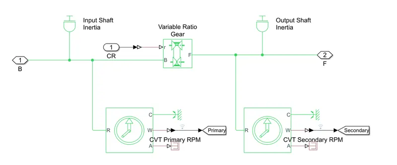
The engine output is connected to a variable ratio gear and the output of the block is given to the simple gear. The variable ratio transmission represents Variable ratio gearboxes include mechanical belt CVTs, electric transmissions, and hydraulic transmissions. The angular shaft velocities input to output ratio is defined by the physical signal input r. Mechanical rotational conserving ports are connections B (base) and F (follower). With the Output shaft rotates parameter, you can specify the relationship between base and follower rotation directions.

The ratio of input and output angular shaft velocities are given by a signal builder block.

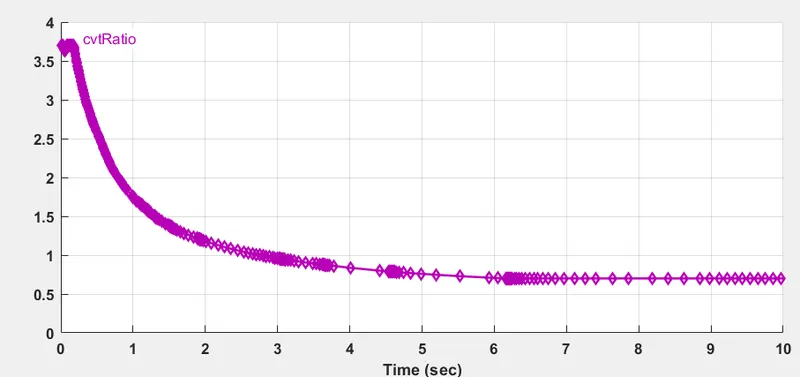
Input and Output shaft inertias are also given which depends on the mass m1 and m2 as 3.5 and 3.2.

Ideal Rotational Motion sensor:

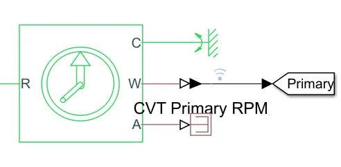
In a mechanical rotational network, this block measures angular velocity or angle. The sensor is perfect since it ignores inertia, friction, delays, energy consumption, and other factors. The angular velocity and angle of port R relative to port C are reported by the physical signal ports W and A, respectively. When the angular velocity at port R is larger than the angular velocity at port C, the observed angular velocity is positive. The output port C is conncected with a mechanical rotational reference. The shaft speed from the primary and secondary are taken from the W port. And the A port is terminated using a PS terminator.

Engine Sensor:

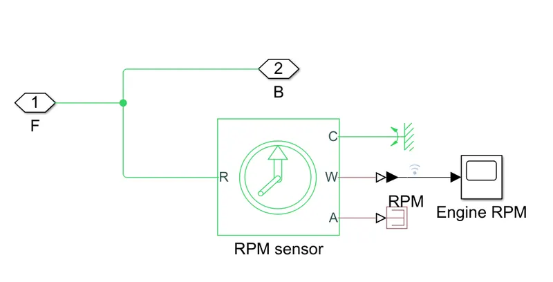
The Engine sensor block is used to display the engine RPM by using a Ideal Rotational Motion sensor.

Generic Engine:

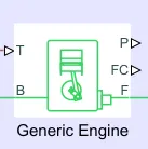
Represents a system-level model of spark-ignition and diesel engines that can be used at the beginning of the modelling process when just the fundamental parameters are known. Idle speed and red line controllers are available as options. The torque needed from the engine is specified as a fraction of the maximum attainable torque via the throttle input signal T, which ranges from zero to one. The engine torque is blended to zero if the engine speed falls below the Stall speed. The simulation will halt and display an error message if the engine speed exceeds the Maximum speed. Mechanical rotational conserving ports F and B are connected to the engine crankshaft and engine block, respectively. Connections P and FC are physical signal output ports through which engine power and fuel consumption rate are reported.

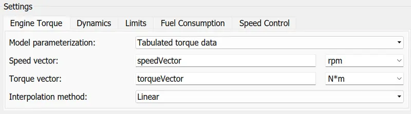
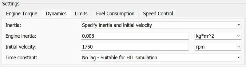
Here port T is connected with the throttle input from signal builder and the B port is connected with the mechanical rotational reference along with a solver configuration.

Brake and Throttle input:

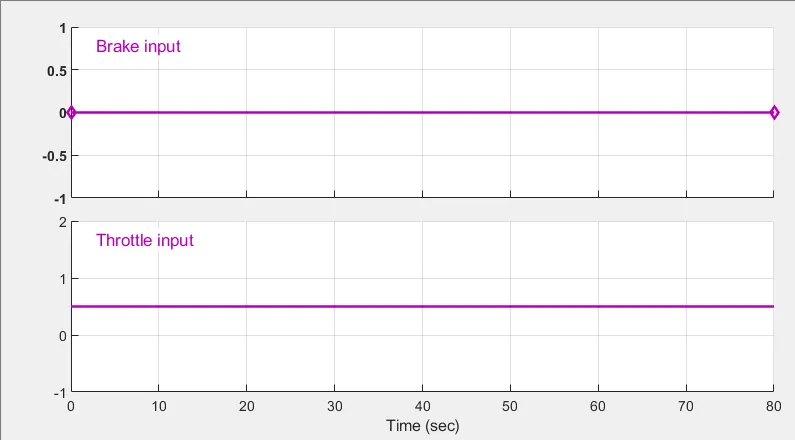
The Brake and Throttle input for the model is given using a signal builder block. Here the brake input is given as zero throughout and throttle input is set to 0.5.

MODEL OF BAJA ATV WITH DASHBOARD:

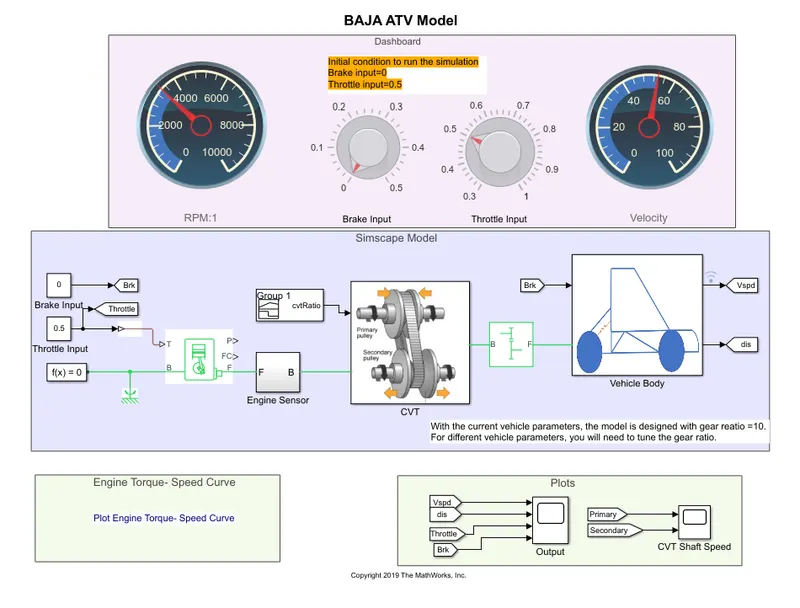
Here the only difference is that the brake and throttle signals from signal buider is changed to Knobs.

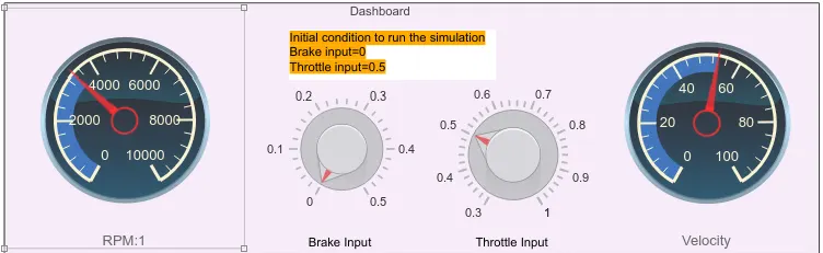
Here the Brake input and Throttle input given below are linked with knobs above, so while giving the stop time as infinity or while the simulation is ongoing we can change the brake and throttle values by just changing the knobs.

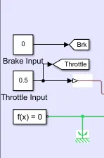
The knobs parameter settings are given as:

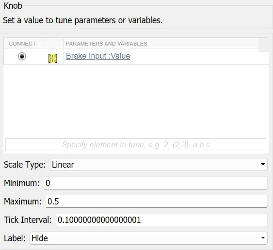
Similarly the dashboard meters are linked with the engine RPM and the velocity speed.

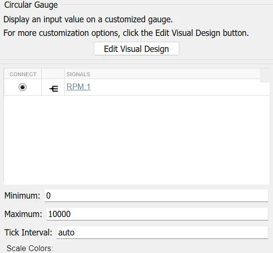
Dashboard blocks just needs to be linked and we need to give the minimum and maximum values for the blocks.

Rest of the model is same as that of without the dashboard. Here the signal builder blocks which provide the input braking and throttle signals are replaced by knobs which can be varied and the speed and rpm outputs are visualized on the meters.

RESULTS:

Engine RPM:

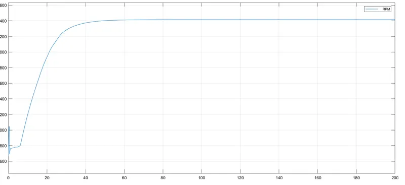
We can see that due to the inertia of the engine shaft there is some variation in speed later on it attains the rpm. At around 50s the engine rpm becomes constant till the stop time and does not reduces since break is not applied.

Vehicle Parameters:

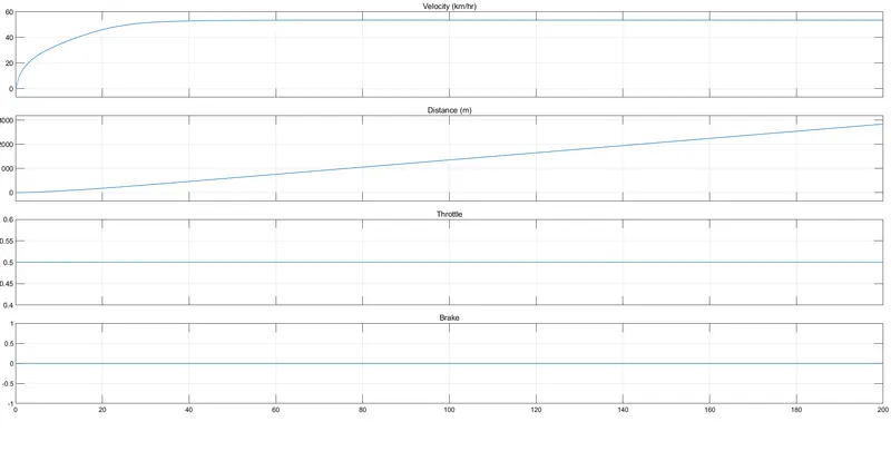
This plot shows the distance covered by the vehicle during the 200s mark. The vehicle attains a constant speed of 50 kmph at around 30s and the distance covered by the vehicle during this period is around 2900m. Input throttle given is a constant value of 0.5 and the brake signal is always zero since no deceleration is done.

CVT Characteristics:

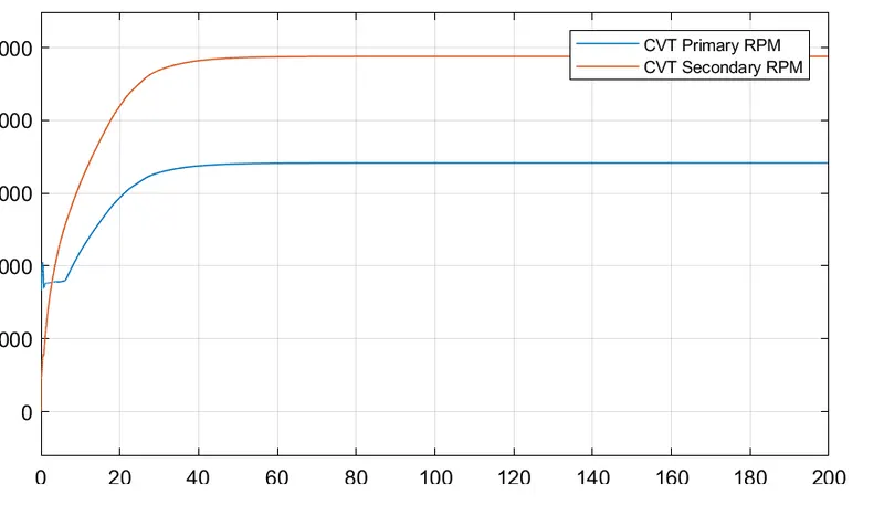
The Speed reduction from input shaft to output can be infered from the plot. Here the input shaft rpm attains around 4800 rpm and the output shaft rpm attained is around 3400 rpm.

Engine Torque-Speed chracteristics:

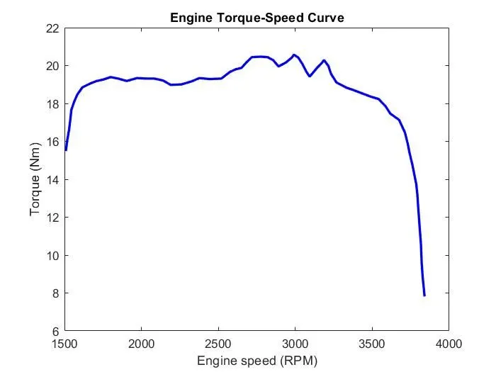
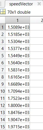
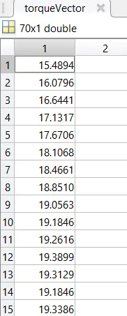
The torque and speed values are given from the matlab workspace to the generic engine to give the output rpm accordingly. The plot is default for all cases as it is the default input to the engine.

Conclusion:

From the plots and engine torque speed characteristics, the vehicle has attained a speed of 45 kmph at the end of 200s stop time and has covered a distance of 2900m. Since there is no braking signal the speed hasnt reduced and the vehicle continue to move with the speed. When the braking knob is set to 0.5 during the simulation time the vehicle speed will reduces if the throttle value doesnt change.