Project
Aim:
Study and research on Baja ATV Model with Continuously Variable Transmission for Open Loop and closed-loop system
modeling in Simulink by using a lookup table.
Objectives:
Study about Baja ATV with Continuously Variable Transmission.
Study about Continuously Variable Transmission system.
Study about the open-loop, closed-loop, a Lookup table in for Baja ATV with CVT model.
Study and analyze the results obtained from all simulations.
Theory:
In this report, we are studying Baja ATV Model with Continuously Variable Transmission. We are studying how to make the Baja ATV
model in Simulink software by using different blocks, so for that let's first study the Baja vehicle with CVT models in detail.
Baja ATV:
- Baja SAE is a Collegiate Design Series competition run by the Society of Automotive Engineers International (SAE International). Teams
of students from universities all over the world design and build small off-road cars. The cars all have engines of the same
specifications. - The goal in Baja SAE racing is to design, build and race off-road vehicles that can withstand the harshest elements of rough terrain. The vehicles used in Baja SAE racing are often similar in appearance to dune buggies. Before 2007, the events were called "Mini Baja."
- There are multiple dynamic events, The dynamic events include hill climbs, sled pulls, maneuverability events, rock crawls, and
suspension & traction events, and the last most important is the endurance event we call this last event the game-changer. - Static events, such as written reports, presentations, and design evaluations are provided by participating teams. This is when the
teams are judged on ergonomics, functionality, and producibility of their cars; ensuring that the final placement of the team does not
rest solely on the vehicle's performance but rather on a combination of static and dynamic events. - Required reports detail the
engineering and design process that was used in developing each system of the team's vehicle, supported with sound engineering
principles.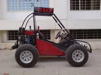
Continuously Variable Transmission(CVT):
Continuously variable transmission (CVT), as its name suggests, continuously varies the gear ratio. A low gear (low ratio) makes it
easier to pull away from a rest position, the drive pulley diameter is relatively small, while the driven pulley diameter is large by
comparison.
The drive belt is possible to select a higher ratio by increasing the diameter of the drive pulley. As acceleration takes place it becomes
possible to select a higher ratio by increasing the diameter of the drive pulley while, at the same time, decreasing the diameter of the
driven pulley. This degree of change can be controlled to ensure that the most suitable ratio is provided. as shown below figure,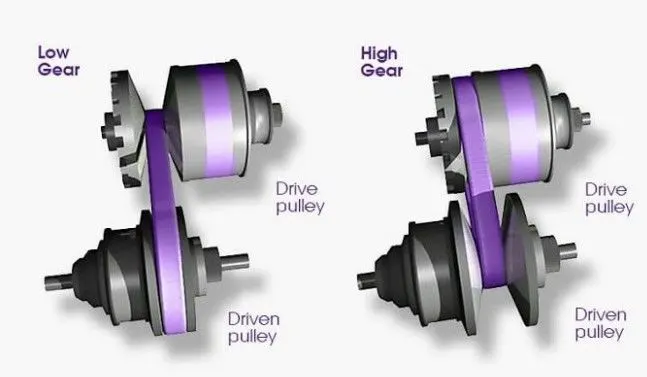
We have a total of two types which we are studying for BAJA ATV with a CVT system model in Simulink which are as follows:
- Open-loop Baja ATV model with CVT system:
- Baja ATV model with CVT system with fixed input to the engine and CVT by the signal builder:
- Baja ATV model with CVT system with variable input to the engine by using variable constant which can be controlled by a knob
and fixed input to CVT by the signal builder:
- Close loop Baja ATV model with CVT system:
- Baja ATV model with CVT system with fixed input to the engine through the step block and input to CVT ratio is selected based on
vehicle speed with the help of lookup table as a close loop system. - Baja ATV model with CVT system with variable input to the engine which can be controlled by knob and input to CVT ratio is
selected based on vehicle speed with the help of lookup table as a close loop system.
- Baja ATV model with CVT system with fixed input to the engine through the step block and input to CVT ratio is selected based on
- Signal Builder: The Signal Builder block allows you to create interchangeable groups of piecewise linear signal sources and use
them in a model. You can quickly switch the signal groups into and out of a model to facilitate testing. In the Signal Builder window,
create signals and define the output waveforms. To open the window, double-click the block.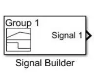
- Generic Engine: The Generic Engine block represents a general internal combustion engine. This block is a suitable generic engine
for spark-ignition and diesel. Speed-power and speed-torque parameterizations are provided. A throttle physical signal input
specifies the normalized engine torque. Optional dynamic parameters include crankshaft inertia and response time lag. A physical
signal port outputs the engine fuel consumption rate based on the fuel consumption model that you choose. Optional speed and
redline controllers prevent the engine to stall and enable cruise control.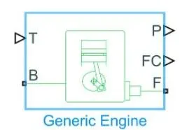
Ports Information:
- T_Port( Normalized engine throttle level, unitless): Engine torque demand as a fraction of maximum possible torque.
- B_Port(Engine block): Mechanical rotational conserving port associated with the engine block. This is the base port. The engine
block is the physical body that contains the piston cylinders. - F_Port(Engine crankshaft): Mechanical rotational conserving port associated with the engine crankshaft. This is the follower port of
the engine. The crankshaft transmits the power generated from the combustion process. Typically, you attach a clutch and
transmission at this port. - P_Port(Instantaneous engine power, W): Power produced by the engine, in W.
- FC_Port(Fuel consumption rate, kg/s): Fuel consumed by the engine, in kg/s.
- Ideal Rotational Motion Sensor:
The Ideal Rotational Motion Sensor block represents an ideal mechanical rotational motion sensor,
that is, a device that converts an across variable measured between two mechanical rotational nodes into a control signal
proportional to angular velocity or angle. You can specify the initial angular position (offset) as a block parameter.
The sensor is ideal since it does not account for inertia, friction, delays, energy consumption, and so on.
Symbol: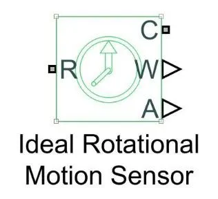
Ports Information:
- R_Port(Rod (positive probe)): Mechanical rotational conserving port associated with the sensor positive probe.
- C_Port(Case (reference probe)): Mechanical rotational conserving port associated with the sensor negative (reference) probe.
- W_Port(Angular velocity, rad/s): Physical signal output port for angular velocity.
- A_Port(Angular displacement, rad): Physical signal output port for angular displacement.
- Variable Ratio Transmission: The Variable Ratio Transmission block represents a gearbox that dynamically transfers motion and
torque between the two connected driveshaft axes, base, and follower.
Symbol: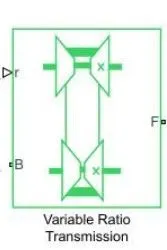
Ports Information:
- B_Port: It is a rotational conserving port representing the primary pully of CVT.
- F_Port: It is a rotational conserving port representing the Secondary pully of CVT.
- r_Port: We specify the unitless variable gear ratio gFB(t) as a function of time at the physical signal input at port r. If the signal
value becomes zero or negative, the simulation stops with an error.
- Simple Gear Box: The Simple Gear block represents a gearbox that constrains the connected driveline axes of the base gear, B, and
the follower gear, F, to corotate with a fixed ratio that we specify. We choose whether the follower axis rotates in the same or opposite
direction as the base axis. If they rotate in the same direction, the angular velocity of the follower, ωF, and the angular velocity of the
base, ωB, have the same sign. If they rotate in opposite directions, ωF and ωB have opposite signs.
Symbol: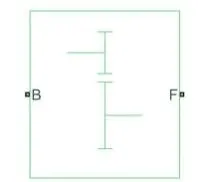
Ports Information:
- B_Port: Rotational mechanical conserving port associated with the base, or input, shaft.
- F Port: Rotational mechanical conserving port associated with the follower or output shaft.
- Vehicle Body: The Vehicle Body block represents a two-axle vehicle body in longitudinal motion. The vehicle can have the same or
a different number of wheels on each axle. For example, two wheels on the front axle and one wheel on the rear axle. The vehicle
wheels are assumed identical in size. The vehicle can also have a center of gravity (CG) that is at or below the plane of travel.
The block accounts for body mass, aerodynamic drag, road incline, and weight distribution between axles due to acceleration and
road profile. Optionally include pitch and suspension dynamics. The vehicle does not move vertically relative to the ground.
The block has an option to include an externally defined mass and an externally defined inertia. The mass, inertia, and center of
gravity of the vehicle body can vary over the course of simulation in response to system changes.
Symbol: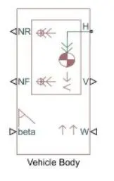
Ports Information:
- W-Port: Physical signal input port for headwind speed.
- beta_Port: Physical signal input port for road incline angle.
- V_Port: Physical signal output port for vehicle longitudinal velocity.
- NF_Port: Physical signal output port for normal force on the front axle. Wheel forces are considered positive if acting downwards.
- NR_Port: Physical signal output port for normal force on the rear axle. Wheel forces are considered positive if acting downwards.
- H_Port: Conserving port associated with the horizontal motion of the vehicle body. Connect tire traction motion to this port.
- Tire(Magic Formula): The Tire (Magic Formula) block models a tire with longitudinal behavior given by the Magic Formula, an
empirical equation based on four fitting coefficients. The block can model tire dynamics under constant or variable pavement
conditions.
The longitudinal direction of the tire is the same as its direction of motion as it rolls on the pavement. This block is a structural
component based on the Tire-Road Interaction (Magic Formula) block.
Symbol: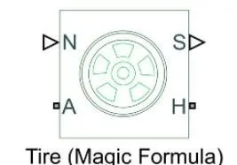
Ports Information:
- N_Port: Physical signal input port associated with the normal force acting on the tire. The normal force is positive if it acts
downward on the tire, pressing it against the pavement. - S_Port: Physical signal output port associated with the relative slip between the tire and road.
- A_Port: Mechanical rotational port associated with the axle that the tire sits on.
- H_Ports: Mechanical translational port associated with the wheel hub that transmits the thrust generated by the tire to the
remainder of the vehicle.
- N_Port: Physical signal input port associated with the normal force acting on the tire. The normal force is positive if it acts
- Double-Shoe Brake: The Double-Shoe Brake block represents a frictional brake with two pivoted rigid shoes that press against a
rotating drum to produce a braking action. The rigid shoes sit inside or outside the rotating drum in a diametrically opposed
configuration. A positive actuating force causes the rigid shoes to press against the rotating drum. Viscous and contact friction
between the drum and the rigid shoe surfaces cause the rotating drum to decelerate.
Double-shoe brakes provide high braking torque with small actuator deflections in applications that include motor vehicles and
some heavy machinery. The model employs a simple parameterization with readily accessible brake geometry and friction
parameters.
Symbol: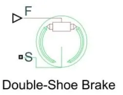
Ports Information:
- F_Port: Physical signal input port associated with the applied actuating force.
- S_Port: Rotational conserving port associated with the rotating drum shaft.
Now let's Discuss all model in brief as follows:
-
- Baja ATV model with CVT system with fixed input to the engine and CVT by the signal builder:
Simulink Model: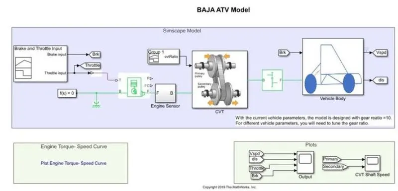
Simulink Model Explanation:
- First step is giving input to the engine with the help of a signal builder. We have one input to the engine which is the throttle, in signal
builder we are giving constant throttle for half-press of the throttle for 80 sec. As we are not considering the Braking condition for the
Vehicle we kept input brake zero. the inputs in the signal builder are as shown in the following figure.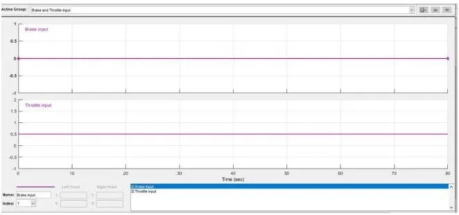
- Now we defined the inputs for the engine, for representing the engine we are using the Generic Engine block which is available in
Simulink. We have to give some parameters of the engine like Speed vector, Torque Vector, Inertia, Idel RPM which is shown in the
below figure.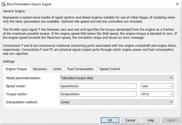
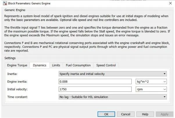
The speed Vector and Torque Vector are the variables defined in the Matlab workspace, the data for speed vector and Torque Vector
is taken from the graph which is as shown in the below diagram with the grabit program.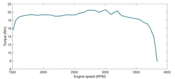
Explanation of the grabit Program is given in references 1 and 2. - Now the output of the engine which is the crankshaft is connected to Ideal Rotational Motion Sensor to measure the RPM of the
engine and plot the graph by using Scope Block. The output of the Engine is also connected to the input shaft(Base) of the Variable
Ratio Transmission which acts as the CVT.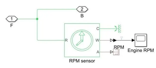
- As we know the output of the engine is connected to the Input shaft which acts as the primary shaft of CVT. As we know that in CVT
there is a continuous change in ratio so for that we have to give input CVT ratios for the given range which depend on the CVT model,
So the Input for Variable ratio transmission block to act as CVT is given with the help of signal builder to the port 'r' as shown in below
graph and diagrams: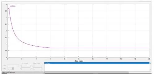
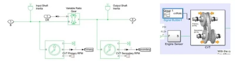
We have defined the inertia for input and output shaft with the help of the following formulas:
for input shaft inertia=`m1*(((18.6e-2)/2)^2+((2.5e-2)/2)^2)/2`
for output shaft inertia=`m2*(((19.8e-2)/2)^2+((1.9e-2)/2)^2)/2`
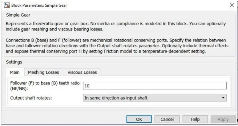
Whereas m1=3.5Kg and m2=3.2Kg which is defined in the MATLAB workspace. We have connected the ideal rotational motion sensor to the input and output shaft i.e. primary and secondary pulley of the CVT to measure the RPM of both pullies to the graph. - Now the output of the CVT i.e. Secondary pulley is connected to the Input of the simple gearbox which is having a gear ratio of 10.
- Last step is to connect the output of the gearbox shaft to the rear wheel of the Baja ATV for which we have to make the Baja ATV
model which is as shown in the diagram: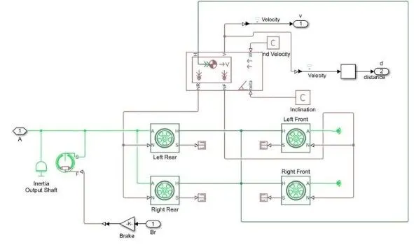
We are considering a rear-wheel-drive system for our BAJA ATV model so we have connected the output of the gearbox to rear
wheels only. we are also connecting double-shoe brake to rear wheels, Now to define the rear wheel and front wheel and other
parameters of the vehicle we are using vehicle body block which is available in Simulink. The input parameters for the vehicle body
are shown in the diagram.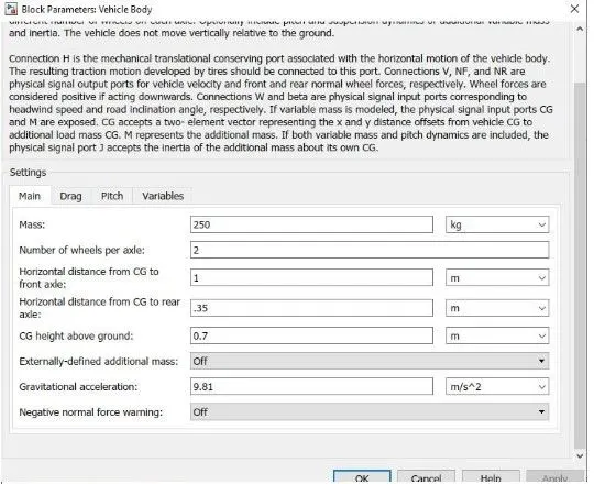
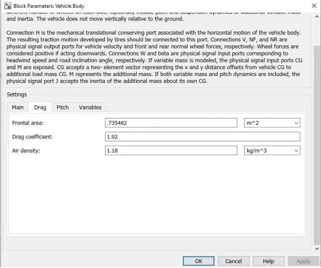
We are considering Headwind speed and inclination plane values zero for this model. The V port is output to get the speed of the
vehicle and to get the distance we connect the integer block to velocity output to get the distance. - Now to plot the outputs we are using Goto and from block to connect the scope.
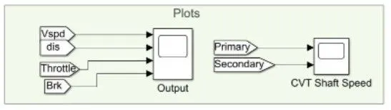
- First step is giving input to the engine with the help of a signal builder. We have one input to the engine which is the throttle, in signal
- Baja ATV model with CVT system with variable input to the engine by using variable constant which can be controlled by a
knob and fixed input to CVT by the signal builder:
Simulink Model: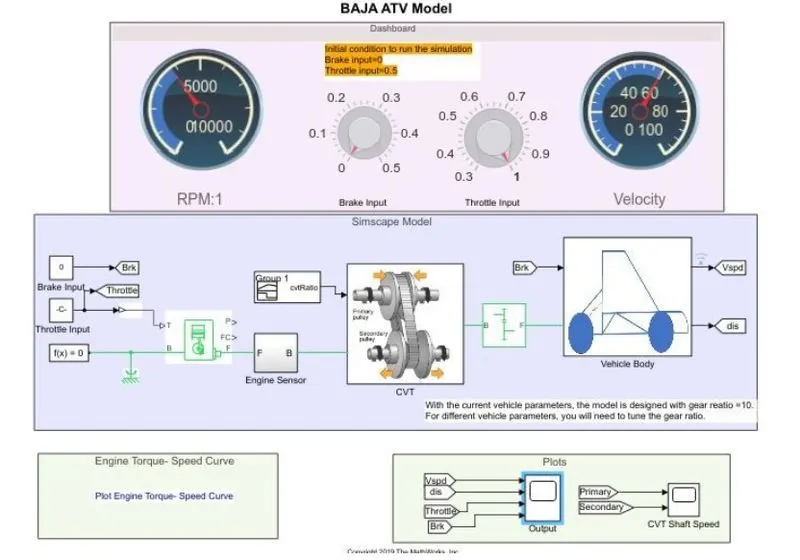
Explanation of the Model:
This model is similar to the above 1.a model but the difference is the only the type of input we are providing which is explained as
follows:
- In this model we can change the input values of throttle and brake with the help of knobs.
- In this model the simulation runtime is kept at infinity so that we can change the values of the throttle and brake during the
simulation run to get the real-time effect of the input parameters. - We also have two circular gauges which are connected to measure the RPM of the engine and velocity of the vehicle as shown in
the above diagram.
- Baja ATV model with CVT system with fixed input to the engine through the step block and input to CVT ratio is selected based
on vehicle speed with the help of lookup table as a close loop system.
Simulink Model: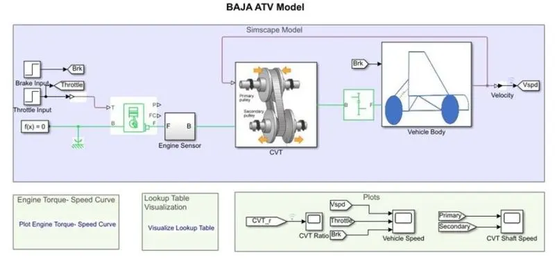
Explanation of the Simulink Model:
- In this model we are giving input to the engine with the help of step blocks. As we know that we are considering only accelerating
conditions so we are keeping the braking condition zero throughout the simulation. the input to the engine with step values is shown
below.
- Throttle input
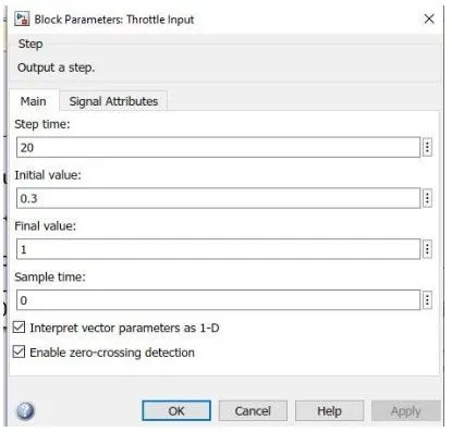
As per these values, the throttle will be pressed 0.3 for 0 to 20 sec and at 20 sec it increases(i.e. it take a step) to the final value which
is 1 for the rest of the simulation time. - Brake input:
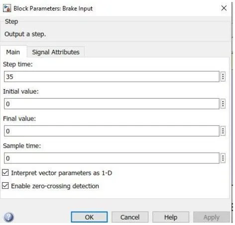
As we can see throughout the simulation time the braking value is zero.
Now the output of the throttle and brake is connected to the GoTo block and connected to the scope block by from block.
- Throttle input
- Now the output of the throttle is connected to the input of the engine. We are using a generic engine with parameters as shown
below diagram: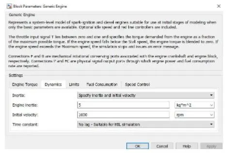
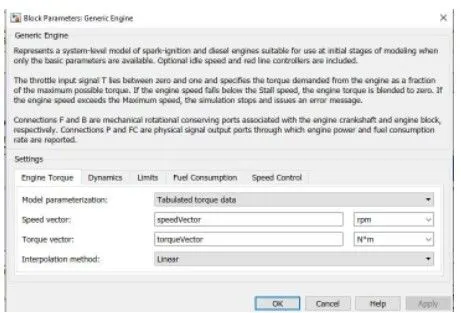
The speed vector and Torque vector are variables defined in the Matlab workspace from the below graph points with the help of the
grabit program.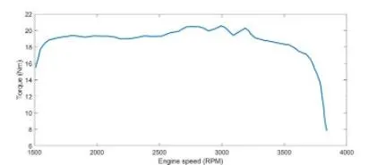
The engine inertia is 5Kg ⋅ m and Idel RPM(i.e. Initial Velocity) is 1600rpm. - Now the output of the engine is connected to the Ideal rotational motion sensor to get the RPM of the engine and next the output of
the engine is connected to the input shaft of the variable ratio transmission(i.e. Primary shaft of the CVT)For the variable CVT ratios
we are using the lookup table.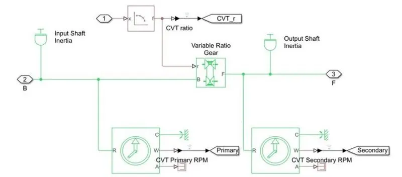
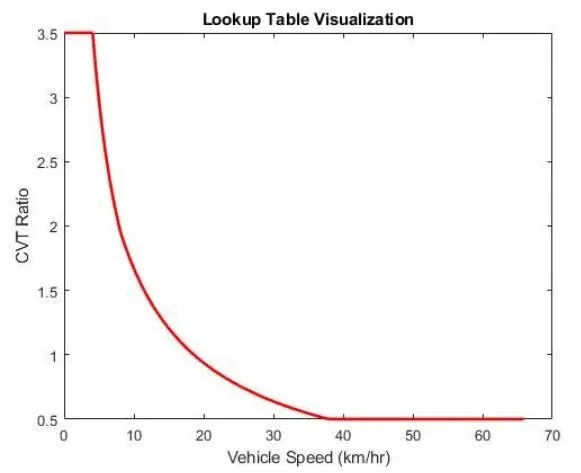
Lookup Table:
We are selecting the CVT ratios according to the velocity of the vehicle which is connected to the input of the Lookup table from the
output of the vehicle model. In the lookup table for input, we are taking vehicle velocity array in increasing order and for output values,
we are taking CVT ratio's, so when we run the simulation CVT changes its ratio according to the vehicle velocity because we have
connected input of lookup table to the output of the vehicle velocity of the vehicle body.
To get the values of Vehicle speed and CVT ratios we used the following Simulink model: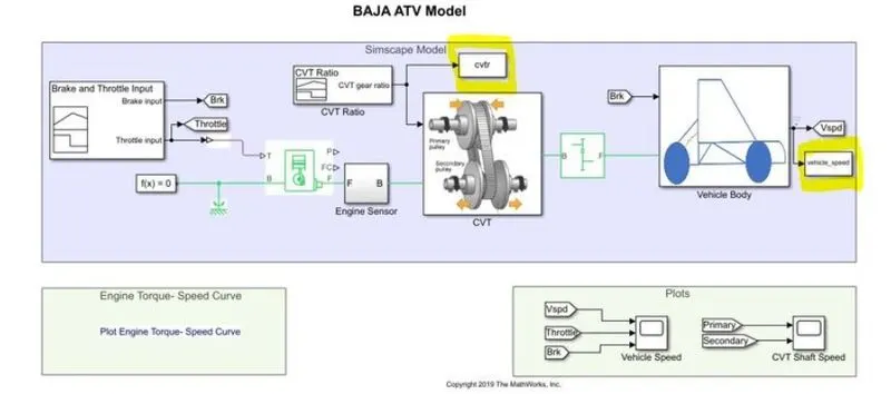
As we can see this model is the same as 1.a model but the only difference is that we have connected 'To Workspace' blocks at the
output of the CVT ratio graph and the output of the Vehicle speed at the vehicle body as shown in above diagram marked with the
yellow marker. These blocks are connected to collect the data to the workspace so we can use that in the Lookup table.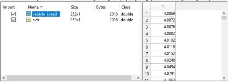
Now the output of the Lookup table is connected to the input of the Variable ratio transmission(i.e. to r port) and also connected to
the GOTO block to get the graph of the output CVT ratios in graph formate. We can also do lookup table parameters visualization by
writing the below program in Matlab.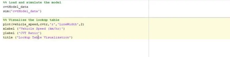
We are using a sim command to open and run the above Simulink model, after completion of the simulation the data of Vehicle
speed and CVT ratio is saved in the workspace so we take this data to plot the graph to do Visualization of the lookup table.
Now we have connected the output of the engine to the input shaft of the Variable ratio transmission and the output shaft of the
Variable ratio transmission is connected to the input of the gearbox. Across these two shafts, we have connected the inertia blocks to
give the inertia and also connected to the ideal rotational motion sensor block to measure the RPM of the primary and secondary
pulley. - Now the output of the secondary pulley is connected to the input shaft of the gearbox. We are using a gearbox with a gear ratio of 12
in this simulation. - Next the output of the gearbox is connected to the both rear wheels of the of Baja ATV because we are considering rear wheel drive
system. and also we have connected double-shoe brake to the rear wheel as shown in diagram: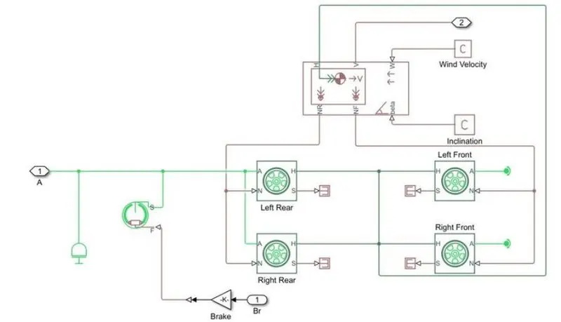
As we can see in above diagram the front wheel(NF) and rear wheels(NR) are defined by using vehicle body block. the all wheels are
connected to the H_port to give only horizontal motion to the wheels. For front wheel we are giving free rotation only. We are not
considering headwind speed and road inclination angle for this model so their values is given zero in constant block. Now the output
port of vehicle body which is speed is connected to the GoTo block to connect it to scope by using from block to plot the graph. - Now to plot the graph we used scope block as shown below:
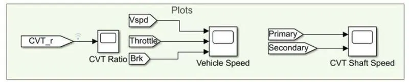
- In this model we are giving input to the engine with the help of step blocks. As we know that we are considering only accelerating
- Baja ATV model with CVT system with variable input to the engine which can be controlled by knob and input to CVT ratio is
selected based on vehicle speed with the help of lookup table as a close loop system.
Simulink Model: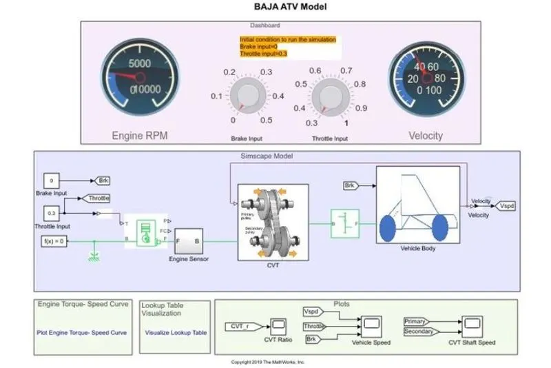
Explanation of the model:
- This model is same as 2.a but the only difference is type of input we are giving to the engine block i.e. it is real time simulator.
- In this model we have connected throttle and brake to engine with the help of constant blocks which are connected to the knob.
- The throttle knob can be varied to the range of 0.3 to 1 and the brake knob can be varied to the range of the 0 to 0.5.
- We also connected circular gauge to measure the engine rpm and the vehicle speed.
- This model is same as 2.a but the only difference is type of input we are giving to the engine block i.e. it is real time simulator.
- Baja ATV model with CVT system with fixed input to the engine and CVT by the signal builder:
Outputs:
-
-
- Baja ATV model with CVT system with fixed input to the engine and CVT by the signal builder
- Graph for the vehicle speed and distance for given value of throttle and brake:
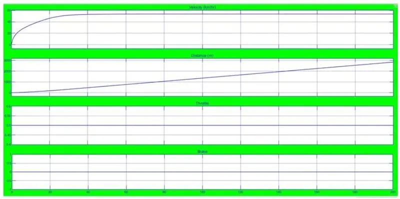
Result:
As we can see that when we press the throttle to 0.5 the vehicle speed increase to its corresponding value with corresponding
distance. - Graph for primary and secondary rpm of the CVT
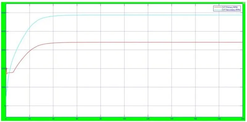
Result:
As we can see that as primary pulley rpm increase the corresponding secondary pulley rpm increase w.r.t. the given cvt
ratios. - Graph of engine RPM:
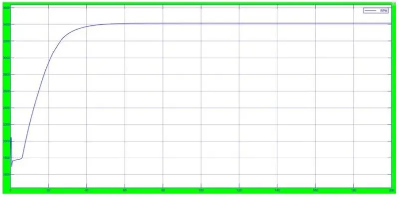
Result:
From the above four graphs we can say that as we press the throttle for 0.5 the engine attends its corresponding rpm, first the
rpm decrease to get the required torque to move the vehicle then it increases w.r.t. time, now next this engine rpm is transferred to
the secondary pulley with the help of the primary pulley. Forgiven vehicle rpm the CVT ratios are selected from the signal builder.
- Graph for the vehicle speed and distance for given value of throttle and brake:
- Baja ATV model with CVT system with variable input to the engine by using variable constant which can be controlled by a knob
and fixed input to CVT by the signal builder
- Graph for change in vehicle speed and distance for given input of throttle and brake.
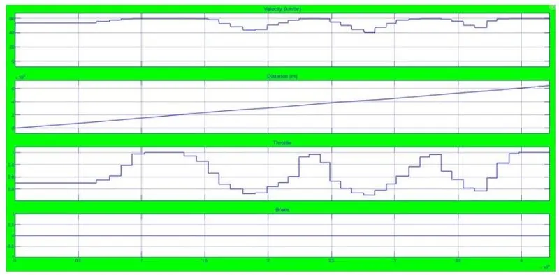
Result:
As we can see that as we change the input throttle values with the help of the knob the corresponding vehicle speed increase
or decreases. - Graph for primary and secondary pullies RPM of CVT:
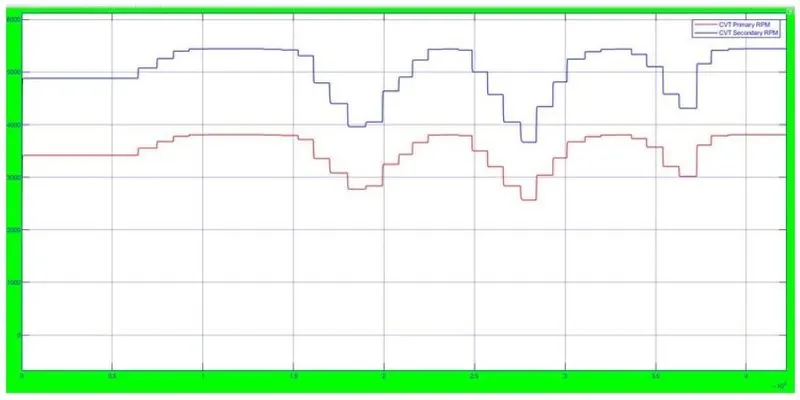
Result:
As we can see that the secondary pulley rpm increases or decreases w.r.t. the primary pulley rpm(i.e. the rpm of the engine)
and the corresponding CVT ratios. - Graph for Engine RPM:
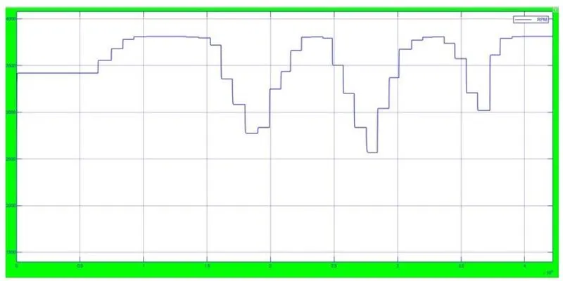
Result: The rpm of the engine changes according to the throttle input.
- Graph for change in vehicle speed and distance for given input of throttle and brake.
- Baja ATV model with CVT system with fixed input to the engine and CVT by the signal builder
-
- Baja ATV model with CVT system with fixed input to the engine through the step block and input to CVT ratio is selected based on vehicle speed with the help of lookup table as a close loop system.
- Graph for vehicle speed with respect to throttle and brake values:
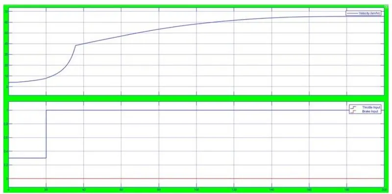
Result:
In this graph the speed increases continuously according to the throttle input and once the throttle input reaches to its
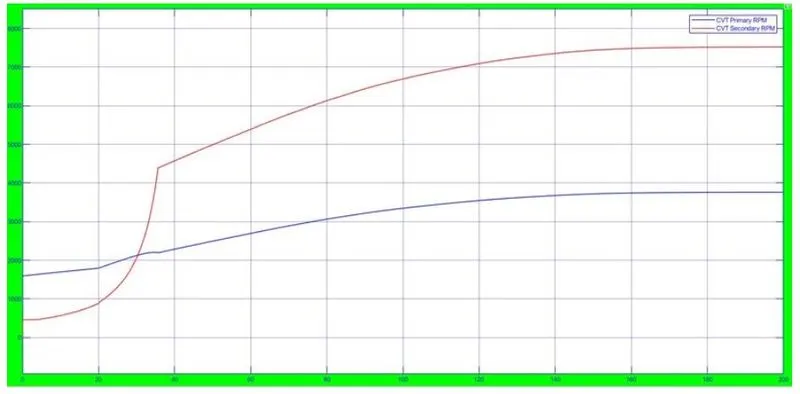
maximum value which is 1 the speed increases to its maximum value. - Graph for primary and secondary pullies RPM of CVT:
Result:
As we can see that the secondary pulley rpm is low for starting time compared to the primary pulley rpm because to get initial
torque required to the move the vehicle. As we are giving input to the CVT w.r.t. vehicle speed by lookup table so when the input speed
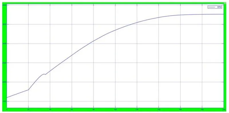
is low it select the required CVT ratio to get required secondary pulley rpm. - Graph for engine rpm:
Result:
As we know that for the first 20sec the throttle input is 0.3 so the engine rpm is low once the engine input throttle jumps to 1
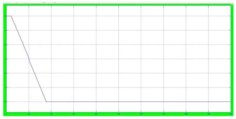
value the engine rpm increases rapidly w.r.t. time. - Graph for CVT ratios:
Result:
As the engine, rpm goes on increasing the CVT ratio decreases to get the required rpm of the CVT secondary pulley. - Graph for CVT ratios from lookup tables:
- Graph for vehicle speed with respect to throttle and brake values:
- Baja ATV model with CVT system with variable input to the engine which can be controlled by knob and input to CVT ratio is
selected based on vehicle speed with the help of lookup table as a close loop system.
- Graph for vehicle speed output with input as throttle and brake
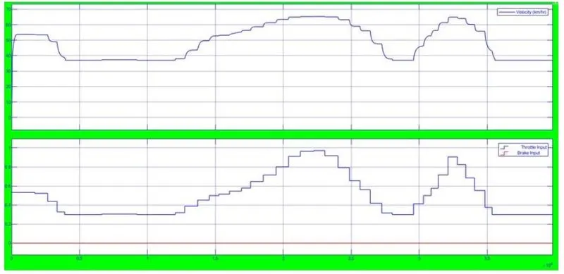
Result:
So as the throttle input to the engine increases or decreases the corresponding vehicle speed increases or decreases
concerning time. - Graph for CVT ratios:
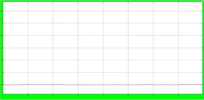
Result:
For the initial simulation time the CVT ratio is high to provide the required torque to the engine once the speed of the
vehicle increases the CVT ratio goes on decreasing, - Graph for engine RPM:
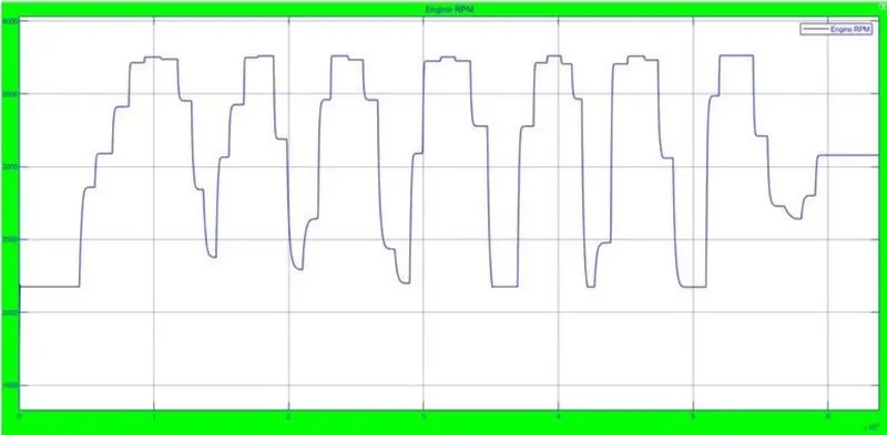
Result: The engine rpm increases or decreases according to the input throttle values. - Graph for primary and secondary pullies RPM of CVT:
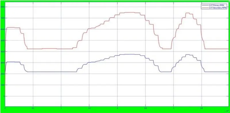
Result:
So for the initial time the secondary pulley rpm increases and after some time it changes according to the primary pulley rpm
and according to the vehicle speed to select the correct CVT reduction ratio from the lookup table.
- Graph for vehicle speed output with input as throttle and brake
- Baja ATV model with CVT system with fixed input to the engine through the step block and input to CVT ratio is selected based on vehicle speed with the help of lookup table as a close loop system.
-
Reference:
https://www.mathworks.com/matlabcentral/fileexchange/70576-baja-all-terrain-vehicle-atv-model
Conclusion:
So from this case we learned how to make Baja ATV model with CVT system using the simulink blocks, Next we learned
how we can use lookup tables to add more realistic conditions for Baja ATV model with CVT system. from the above
graph we can also adjust the gear ratio or CVT ratio for different conditions instead of trying to do on real model which
take more time we can do same using simulink model within the minute. As we can also plots the graph of different
outputs we can adjust the ratios of the both CVT and gearbox, we can get the required tuning for required track
conditions