Week 4.1 - Genetic Algorithm
AIM: Write a code in MATLAB to optimise the stalagmite function and find the global maxima of the function.
THEORY:
Global Algorithm:
The genetic algorithm repeatedly modifies a population of individual solutions. At each step the genetic algorithm selects individuals at random from the each current population to be parents and uses them to produce the children for the next generation.
The genetic algorithm uses three main types of rules at each step to create the next generation from the current population:
- Selection rules select the individuals called parents, that contribute to the population at the next generation.
- Crossover rules combine twp parents to form children for the next generation.
- Mutation rules apply random changes to individual parents to form children.
"Syntax For GA"
FitnessfcnFitness Functions|
nvars |
Number of design variables |
|
Aineq |
A matrix for linear inequality constraints |
|
Bineq |
b vector for linear inequality constraints |
|
Aeq |
Aeq matrix for linear equality constraints |
|
Beq |
beq vector for linear equality constraints |
| lb |
Lower bound on x |
|
ub |
Upper bound on x |
| nonlcon |
Nonlinear constraint function |
| rngstate | Optional field to reset the state of the random number generator |
| solver | ga |
| options | Options created using optimoptions or expotred from the optimization app |
x = ga(fun,nvars) finds a local unconstrained minimum, x, to the objective function, fun. nvars is the dimension (number of design variables) of fun.x = ga(fun,nvars,A,b,Aeq,beq,lb,ub,nonlcon)nonlcon. The function nonlcon accepts x and returns vectors C and Ceq, representing the nonlinear inequalities and equalities respectively. ga minimizes the fun such that C(x) ≤ 0 and Ceq(x) = 0. (Set lb=[] and ub=[] if no bounds exist.)
[ also returns a matrix x,fval,exitflag,output,population,scores] = ga(___)population, whose rows are the final population, and a vector scores, the scores of the final population.
PROGRAM:
% Defining our search space to be optimized.
% Creating One dimensional array
x= linspace(0,0.6,150);
y= linspace(0,0.6,150);
num_cases = 60;
% Creating two dimensional arrays from one dimensional array
[xx,yy]= meshgrid(x,y);

% Evaluating the stalagmite function

for i= 1:length(xx)
    for j= 1:length(yy)
        input_vector(1)= xx(i,j);
        input_vector(2)= yy(i,j);
        f(i,j)= stalagmite_fun(input_vector);
    end
end

surf(xx,yy,f)
shading interp

xlabel('x value')
ylabel('y value')
[x_output,fval]= ga(@stalagmite_fun,2);
Inputs X and Y are assigned by using linspace command and afterwards 2 dimensional array is generated by using meshgrid command. "forloop" command is used for repetitive vector data formation and executed by calling hyperlinked function code fot stalagmite.
Function Code:
function [stalagmite]= stalagmite_fun(input_vector)
x= input_vector(1)
y= input_vector(2)
f1_x = (sin(5.1*pi*x+0.5)).^6;
f2_y = (sin(5.1*pi*y+0.5)).^6;
f3_x = exp((-4*0.6931).*(x-0.0667)^2/(0.64));
f4_y = exp((-4*0.6931).*(y-0.0667)^2/(0.64));
stalagmite = (f1_x.*f2_y.*f3_x.*f4_y)
end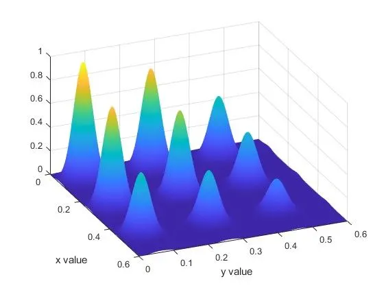
% Defining our search space to be optimized.
% Creating One dimensional array
x= linspace(0,0.6,150);
y= linspace(0,0.6,150);
num_cases = 60;
% Creating two dimensional arrays from one dimensional array
[xx,yy]= meshgrid(x,y);

% Evaluating the stalagmite function

for i= 1:length(xx)
    for j= 1:length(yy)
        input_vector(1)= xx(i,j);
        input_vector(2)= yy(i,j);
        f(i,j)= stalagmite_fun(input_vector);
    end
end

% Study1 Statistical Behaviour
tic
for i = 1:num_cases
[inputs,fopt(i)]= ga(@stalagmite_fun,2);
xopt(i)= inputs(1);
yopt(i)= inputs(2);
end
study_time_1= toc;

% Plotting
figure(1)
subplot(2,1,1);
hold on
surfc(xx,yy,f);
shading interp

xlabel('x data');
ylabel('y data');
plot3(xopt,yopt,fopt,'Marker','o','MarkerSize',3,'MarkerFaceColor','r');
title('Unbounded Inputs')
subplot(2,1,2)
plot(fopt)
xlabel('Iterations')
ylabel('Maximum Function')


% Study2 Bounded Inputs

tic
for i= 1:num_cases
    [inputs,fopt(i)]= ga(@stalagmite_fun,2,[],[],[],[],[0,0],[1,1]);
    xopt(i) = inputs(1);
    yopt(i) = inputs(2);
end
study_time_2=toc;

figure(2)
subplot(2,1,1)
hold on
surfc(xx,yy,f)
shading interp
xlabel('X data')
ylabel('Y data')
plot3(xopt,yopt,fopt,'Marker','o','MarkerSize',3,'MarkerFaceColor','g');
title('Bounded Inputs')
subplot(2,1,2)
plot(fopt)
xlabel('Iterations')
ylabel('Maximum Function')


% Study3 Bounding the valuesand increasing population size

options = optimoptions('ga');
options = optimoptions(options,'PopulationSize',300);
tic
for i= 1:num_cases
    [inputs,fopt(i)]= ga(@stalagmite_fun,2,[],[],[],[],[0,0],[1,1],[],[],options);
    xopt(i)= inputs(1);
    yopt(i)= inputs(2);
end

study_time_3= toc

figure(3)
subplot(2,1,1)
hold on
surfc(xx,yy,f)
shading interp
xlabel('X data')
ylabel('Y data')
plot3(xopt,yopt,fopt,'Marker','o','MarkerSize',3,'MarkerFaceColor','g');
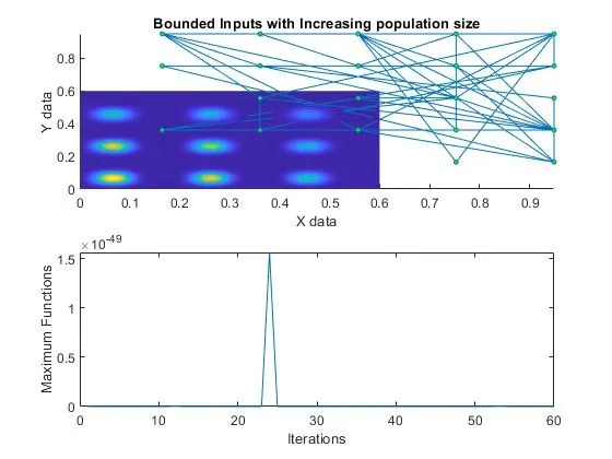
title('Bounded Inputs with Increasing population size');
subplot(2,1,2)
plot(fopt)
xlabel('Iterations');
ylabel('Maximum Functions');
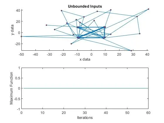
Case Study 1: Unbounded inputs
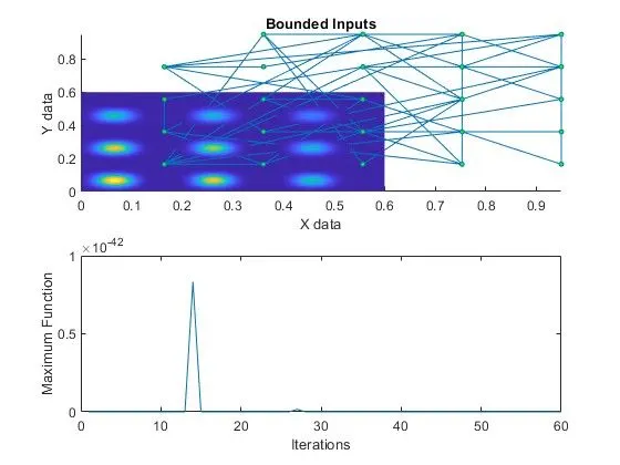
Case Study 2: Bounded the values
Case Study 3: Bounded inputs with increased population size
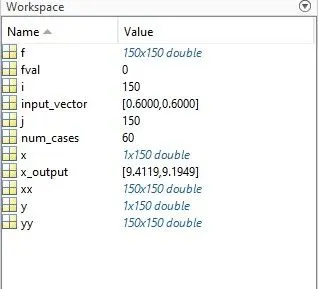
Workspace Data:
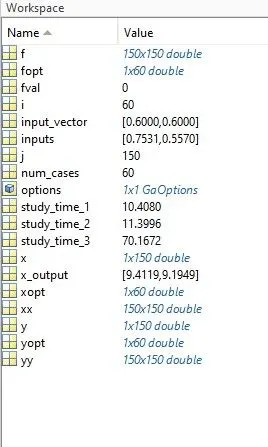
Presented results shows data from 3 experimented investigations to examine statistical behavior which shows optimization of code has been done.
REFERENCE:
https://www.iitg.ac.in/rkbc/CE602/CE602/Genetic%20Algorithms.pdf
https://in.mathworks.com/videos/what-is-a-genetic-algorithm-100904.html