Project 2 - Rankine cycle Simulator

Aim: To simulate the Rankine Cycle and plot the corresponding T-S and H-S plots using MATLAB.

Objective:

1. Calculate the state points of the Rankine Cycle based on given inputs.
2. Plot the corresponding T-S and H-S plots for the given set of inputs.

Given:
Input Values:

1. Turbine Inlet temperature = 400° C
2. Turbine Inlet Pressure = 30 bars
3. Turbine Outlet Pressure = 0.05 bars = Condenser Inlet Pressure

Required Output Values:

1. Net work output (Wnet)
2. Back work ratio (BWR)

"Note: The standard Xsteam library is used to get the steam table data for water is given, which is used to calculate the points in between the state variables."

Introduction:

1. Rankine cycle converts thermal energy to mechanical energy.
2. On-road vehicles, which convert around one-third of the fuel energy into useful mechanical energy for propulsion, are moving
   energy conversion systems that generate considerable waste heat.
3. It is found from prior research that the Rankine Cycle has great potential in automobile waste heat harvesting applications
   which can, in turn, be connected to the combustion engine which will result in better-wasted heat consumption and increasing
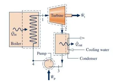
   the performance of the vehicle and helping the environment.
4. Rankine cycle is the most basic thermodynamic cycle for any steam powerplant. It starts with the heating of water in the boiler
   at constant pressure to produce steam. The steam produced is then isentropically expanded in the turbine to produce work.
   After the turbine, the steam goes into the condenser where it is cooled and converted into the water at constant pressure. The
   water is then again pumped back to the boiler by a pump and the cycle continues.
5. The ideal Rankine cycle consists of the following four processes:
   1. 1-2: Isentropic compression in a pump
   2. 2-3: Constant pressure heat addition in a boiler
   3. 3-4: Isentropic expansion in a turbine
   4. 4-1: Constant pressure heat rejection in a condenser

Procedure:

1. First, all the required variables and parameters were found out to calculate.
2. Then, using the ‘XSteam’ library function, all the parameters were sorted out.
3. Then, the usual calculations and plotting of the graphs were done as per the theory of thermodynamics.

MATLAB Program:

% Rankine Cycle Simulator
clear all
close all
clc

% Basic information
fprintf('RANKINE CYCLE SIMULATOR \n')
fprintf('\n1-2 is isentropic expansion in the Turbine \n')
fprintf('2-3 is Constant pressure Heat rejection by condenser \n')
fprintf('3-4 is isentropic compression in pump \n')
fprintf('4-1 is constant pressure heat addition by the boiler \n')

% User inputs
P1 = input('\n Enter the pressure at the Turbine inlet (in bar): ');
T1 = input('\n Enter the temperature at the Turbine inlet (in Degree Celcius): ');
P2 = input('\n Enter the pressure at the Turbine outlet (in bar): ');

% State Point 1
H1 = XSteam('h_pt',P1,T1);  % Enthalpy
S1 = XSteam('s_pt',P1,T1);  % Entropy
Hf1 = XSteam('hL_p',P1);    % Enthalpy of saturated liquid
Hg1 = XSteam('hV_p',P1);    % Enthalpy of saturated vapour
Ts1 = XSteam('Tsat_p',P1);  % Saturation Temperature
Sf1 = XSteam('sL_p',P1);    % Entropy of saturated liquid
Sg1 = XSteam('sV_p',P1);    % Entropy of saturated vapour

% State point 2
S2 = S1;
Sf2 = XSteam('sL_p',P2);
Sg2 = XSteam('sV_p',P2);
x = (S2-Sf2)/(Sg2-Sf2); % Dryness fraction
Hf2 = XSteam('hL_p',P2);
Hg2 = XSteam('hV_p',P2);
H2 = Hf2 + x*(Hg2-Hf2);
T2 = XSteam('T_ph',P2,H2);
Ts2 = XSteam('Tsat_p',P2); 

% State point 3
H3 = Hf2;
S3 = Sf2;
T3 = T2;
P3 = P2;

% State point 4
P4 = P1;
S4 = S3;
H4 = XSteam('h_ps',P4,S4);
T4 = XSteam('T_ps',P4,S4);
t = linspace(0,374,500); % temp space for plotting saturation cutves

%Plot T-S Diagram
figure(1)
hold on
% Plot Saturation Curve
for i = 1 : length(t)
 plot(XSteam('sL_T',t(i)),t(i),'.','color','b')
 plot(XSteam('sV_T',t(i)),t(i),'.','color','b')
end

% Plot Cycle
plot([S1 S2],[T1 T2],'linewidth',2,'color','r')
if x>1
 T3 = Ts2;
 plot([S2 Sg2 S3 S4],[T2 Ts2 T3 T4],'linewidth',2,'color','r')
 T2 = Ts2;
else
 plot([S2 S3 S4],[T2 T3 T4],'linewidth',2,'color','r')
end
l = linspace(T1,T2,1000);
for i = 1 : length(l)
 plot(XSteam('s_pT',P1,l(i)),l(i),'.','color','r')
end
plot([Sf1 Sg1],[Ts1 Ts1],'linewidth',2,'color','r')
xlabel('Entropy[KJ/Kg-K]')
ylabel('Temprature[K]')
title('T-S Diagram')

% Plot H-S Diagram
figure(2)
hold on
% Plot Saturation Curve
for i = 1 : length(t)
 plot(XSteam('sL_T',t(i)),XSteam('hL_T',t(i)),'.','color','b')
 plot(XSteam('sV_T',t(i)),XSteam('hV_T',t(i)),'.','color','b')
end

% Plot Cycle
plot([S1 S2 S3 S4 S1],[H1 H2 H3 H4 H1],'linewidth',2,'color','r')
xlabel('Entropy[KJ/Kg-K]')
ylabel('Enthalpy[KJ/Kg]')
title('H-S Diagram')

% calculations
% Turbine Work
Wt = H1-H2;

% Pump Work
Wp = H4-H3;

% Heat Addition
Qin = H1-H4;

% Heat Rejection
Qout = H2-H3;

% Net Work
Wnet = Wt-Wp;

% Efficiency
Ntherm = (Wnet/Qin)*100;

% Specific steam consumption
SSC = 3600/Wnet;

% Back Work Ratio
BWR = Wp/Wt;

% Print Results
fprintf('\n\nResults\n')
fprintf('At State Point 1:\n')
fprintf('P1 is : %.2f bar\n',P1)
fprintf('T1 is : %.2f Deg Celcius\n',T1)
fprintf('H1 is : %.2f KJ/Kg\n',H1)
fprintf('S1 is : %.2f KJ/Kg-K\n',S1)

fprintf('\nAt State Point 2:\n')
fprintf('P2 is : %.2f bar\n',P2)
fprintf('T2 is : %.2f Deg Celcius\n',T2)
fprintf('H2 is : %.2f KJ/Kg\n',H2)
fprintf('S2 is : %.2f KJ/Kg-K\n',S2)

fprintf('\nAt State Point 3:\n')
fprintf('P3 is : %.2f bar\n',P3)
fprintf('T3 is : %.2f Deg Celcius\n',T3)
fprintf('H3 is : %.2f KJ/Kg\n',H3)
fprintf('S3 is : %.2f KJ/Kg-K\n',S3)

fprintf('\nAt State Point 4:\n')
fprintf('P4 is : %.2f bar\n',P4)
fprintf('T4 is : %.2f Deg Celcius\n',T4)
fprintf('H4 is : %.2f KJ/Kg\n',H4)
fprintf('S4 is : %.2f KJ/Kg-K\n',S4)

fprintf('\nWt is : %.2f KJ/Kg\n',Wt)
fprintf('Wp is : %.2f KJ/Kg\n',Wp)
fprintf('Wnet is : %.2f KJ/Kg\n',Wnet)
fprintf('Thermal Efficiency is : %.2f percent\n',Ntherm)
fprintf('S.S.C. is : %.2f Kg/KWh\n',SSC) 
fprintf('Back Work Ratio is : %.3f \n',BWR)

Steps:

1. Start the program with 'clear all','close all', and 'clc' command.
2. As our task is to take user input, to facilitate users to continue or end the program, we have introduced a while statement at the
   start of the script. While statement, the first step is to make provision for MatLab to accept user input. 'input()' is used to provide the
   user input. The user input includes temperature and pressure before entry to the turbine and pressure after exiting to the turbine.
3. Now based on user inputs parameters at 4 state points are calculated. Thermodynamic parameters include enthalpy H, entropy S,
   temperature T, pressure P, and dryness factor X at state point 2. For calculating these parameters XSteam() i.e. steam table MATLAB.
   program is used. This program consists of functions for all thermodynamic properties. After calling these functions in the main script
   gives us thermodynamic properties based on other properties like temperature and pressure.
4. After calculating all parameters, the next objective is to calculate pump work, turbine work, net work output, back ratio, and
   thermal efficiency.
5. Now, we need to display all these results in the command window which is done by using command 'fprintf()'.
6. The next objective is to plot the graph for H-S and T-S. The first step in plotting this graph is to plot the saturation curve which is
   calculated using 'for' loop. Under 'for' loop, values for entropy and enthalpy are calculated over a temperature range. Plotting these
   calculated values, the plot of a saturation curve can is obtained. Other processes are plotted by plotting respective values of H, S, T.
7. Now, when the program is run it asks the user to input Turbine Inlet temperature, Turbine Inlet Pressure, Turbine Outlet Pressure
   which is Condenser Inlet Pressure.
8. After the input parameters are given, all the results are displayed in the command window.

Results:

1. First, the user has to input the given input parameters in the command window.

• Turbine Inlet temperature = 400° C
• Turbine Inlet Pressure = 30 bars
• Turbine Outlet Pressure = 0.05 bars = Condenser Inlet Pressure

Command Window:

RANKINE CYCLE SIMULATOR 

1-2 is isentropic expansion in the Turbine 
2-3 is Constant pressure Heat rejection by condenser 
3-4 is isentropic compression in pump 
4-1 is constant pressure heat addition by the boiler 

 Enter the pressure at the Turbine inlet(in bar): 30

 Enter the temperature at the Turbine inlet(in Deg celcius): 400

 Enter the pressure at the Turbine outlet(in bar): 0.05


Results
At State Point 1:
P1 is : 30.00 bar
T1 is : 400.00 Deg Celcius
H1 is : 3231.57 KJ/Kg
S1 is : 6.92 KJ/Kg-K

At State Point 2:
P2 is : 0.05 bar
T2 is : 32.88 Deg Celcius
H2 is : 2110.71 KJ/Kg
S2 is : 6.92 KJ/Kg-K

At State Point 3:
P3 is : 0.05 bar
T3 is : 32.88 Deg Celcius
H3 is : 137.77 KJ/Kg
S3 is : 0.48 KJ/Kg-K

At State Point 4:
P4 is : 30.00 bar
T4 is : 32.95 Deg Celcius
H4 is : 140.76 KJ/Kg
S4 is : 0.48 KJ/Kg-K

Wt is : 1120.86 KJ/Kg
Wp is : 3.00 KJ/Kg
Wnet is : 1117.87 KJ/Kg
Thermal Efficiency is : 36.17 percent
S.S.C. is : 3.22 Kg/KWh
Back Work Ratio is : 0.003 
>> 

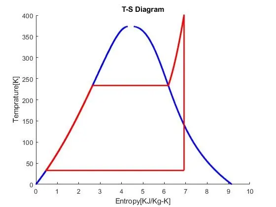
Rankine T-S Diagram:

Rankine H-S Diagram:

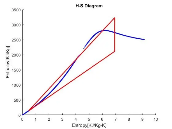
• Here in both the plots, the Blue Curve represents the Saturation Curve, and the Red Curve Represents Cycle.

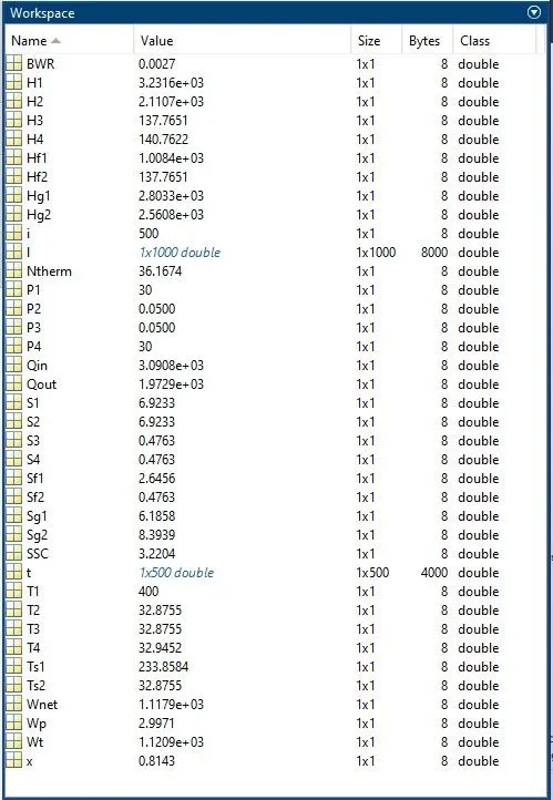
Workspace Values:

Errors found while Programming:

No complicated errors occurred while running the MATLAB program.

Conclusion:

• Rankine cycle is the basic cycle for understanding about the steam turbine systems in thermodynamics.
• The required output values are obtained for the given input parameters:
  • Net work output = 1117.87 KJ/Kg
  • Back work ratio = 0.003
• Thus, the Rankine cycle is successfully simulated using MATLAB.

References:

1. http://www.ecourses.ou.edu/cgi-bin/ebook.cgi?topic=th&chap_sec=10.1&page=theory