Week 3 - Solving second order ODEs

Aim: To plot a graph of Simple Pendulum motion and create an animation of its motion

Theory:

A Simple Pendulum

A simple pendulum is a point mass attached to a string suspended at fixed support. A verticle line passing through the fixed support is called as a mean position of simple pendulum.

The length of the string is the virticle distance from the centre of mass of body when it is at mean position of pendulum.

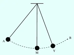
Fig. Diagram of Simple pendulum

Motion of pendulum:

The motion exhibited by the simple pendulum is called as Simple Harmonic Motion.

Simple harmonic motion is a special type of periodic oscillations where the restoring force is directly proportional to the displacement and direction is opposite to that of displacement.

Period of Oscillations:

The period of swings of a simple pendulum depends upon its length , local strength of gravity, and to a small extend on the maximum angle that the pendulum swings away from vertical is called as Amplitude.

The oscillations of the pendulum is also influenced by a factor called Damping.

Damping:

Damping is an influence within or upon an oscillatory system that has the effect of reducing, restricting,its oscillations.

In mechanical system, damping is caused due to viscous drag, fluid density etc. which causes resistance of motion/ oscillations of the object.

Damping coefficient:

A damping coefficient is a material property that indicates whether a material will bounce back or return energy to a system with unit of N.s/m.

Ordinary Differential Equation(ODE)

An ordinary differential equation in mathematics is a differential equation containing one or more fuctions of one independent and the derivatives of those functions. The term ordinary is used in contrast with the term partial differential equation which may be with respect to more than one independent variable.

A first order differntial equation is an equation

dy/dx= f(x,y)

inwhich f(x,y) is a function of two variables defined on a region in the xy plane. The equation is first order because it involves only the first derivative dy/dx.

Note: When the derivatives inincreases in a equation from the previous derivative it becomes higher order equation.

ODE for Simple Pendulum:

Let us consider a ODE representing the equation of motion of a simple pendulum with damping. This is an example of an second order ODE.

d(theta)^2/dt^2+(b/m)*d(theta)/dt+(g/l)sin(theta)=0

In the above equation

b= Damping coefficient

g= gravitational acceleration(m/s^2)

l= length of the pendulum(m)

m= mass of the body(kg)

Using the above equation , we can simulate the motion of a simple pendulum in MATLAB.

Considerations:

1. Using a operator called (ode45), we can solve the equation to get the values. But the operator can solve only first order equation.
2. So we are consideration the second order equation into two first order equation for solving
3. From the equation, First- d(theta1)/dt=theta2
4. Second- d(theta2)/dt+(b/m)theta2+(g/l)sin(theta1)=0

Program: To simulate the motion of the simple pendulum and animate it.

% ODE equation for Pendulum
clear all
close all
clc

% Defining inputs
b=0.05;
g=9.81;
l=1;
m=1;

% Initial conditions
% [angular displacement, angular velocity]
theta_0=[0;3];

% Time points
t_span=linspace(0,20,200);

% Solve ODE equation
[t, results]= ode45(@(t,theta) ode_func(t,theta,b,g,l,m),t_span,theta_0);

% Plotting
figure(1)
% result(:,1) considers all the values on the result in angular
% displacements
plot(t, results(:,1))
hold on
% result(:,2) considers all the values on the result in angular
% velocities
plot(t,results(:,2))
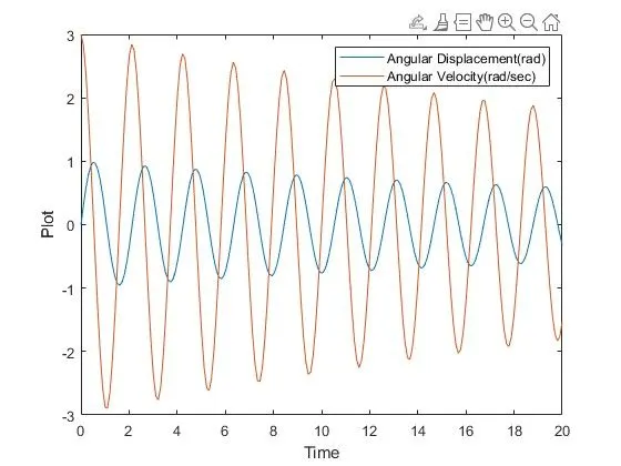
ylabel('Plot')
xlabel('Time')
legend('Angular Displacement(rad)','Angular Velocity(rad/sec)')
% This is the graph for the motion of simple pendulum

% For Animation of simple pendulum
x=1;
for i=1:length(t_span)
    % To find the new coordinates of x from the given time
    x_new= l*sin(results(i,1));
    % To find the new coordinates of y from the given time
    y_new= l*cos(results(i,1));


    figure(2)
    % To plot the line at which the string of pendulum is attached 
    plot([-2.5 2.5],[0 0], 'LineWidth',3,'Color','b')
    hold on

    % Varying x,y points are plotted by using loop command and connected
    % with line as a 'string'
    plot([0 x_new],[0 y_new],'linewidth',2,'color',[0.2 0.2 0.2])
    
    plot(x_new,y_new,'Markersize',20,'MarkerFaceColor','b','MarkerEdgeColor','r')
    axis([-5 5 -5 5])
    pause(0.03)
    hold off 
    % To create a movie using an array of values
    M(x)=getframe(gcf);
    % Increament in frame
    x=x+1;
end

movie(M)
video_pendulum= VideoWriter('C:UsersSaurabhDocumentsMATLABMotion of Simple Pendulum.avi',"Uncompressed AVI");
open(video_pendulum)
writeVideo(video_pendulum,M)
close(video_pendulum)

Program of the function which is called for solving (ode_func)

function [dtheta_dt]= ode_func(~,theta,b,g,l,m)

theta1= theta(1);
theta2= theta(2);
dtheta1_dt= theta2;
dtheta2_dt= -(b/m)*theta2-(g/l)*sin(theta1);
dtheta_dt= [dtheta1_dt; dtheta2_dt];

end

Output:

The below shows the graphical reprsentation of the harmonic motion of the simple pendulum.

Animation Video:

https://drive.google.com/file/d/1dbvOEN760Ts79dkcYQ9QkvWj3G76hAco/view?usp=sharing