Project
Note: The model is downloaded from below link
https://www.mathworks.com/matlabcentral/fileexchange/70576-baja-all-terrain-vehicle-atv-model
Aim: The aim of this project is to understand the modelling and behaviour of All Terrain Vehicle (ATV) using Continuously Variable Transmission (CVT) by simscape and simscape driveline model
Theory
ATV : All-terrain vehicle is open vehicle with single seat with three or more wheels fitted with large tyres for the use on rough ground.
CVT : Continuously variable transmission is used in vehicle to provide different gear ratios over wide range of speed. This helps in keeping engine RPM constant with varying vehicle speed.
The most common CVT is made by using two pulleys driven by belt drive.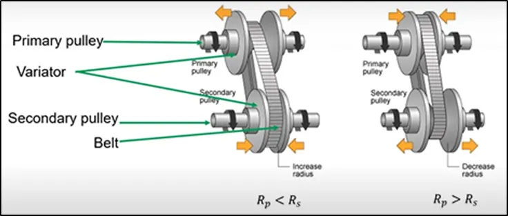
Here as shown in the above image when pulleys goes outward then radius decreases and when goes inward, then radius increases. Rp<Rs causes speed reduction and Rp>Rs causes overdrive.
Following are the major common components used in all the model
- Signal Builder:
It is used to provide brake and throttle input. The two signals are made in signal builder. Brake input is given to vehicle body and throttle input to engine.
- Generic Engine:
It is used to represent the physical model of IC engine which is driven by throttle input as demand of torque.
Port F & B are mechanical rotational conserving ports associated with engine crankshaft.
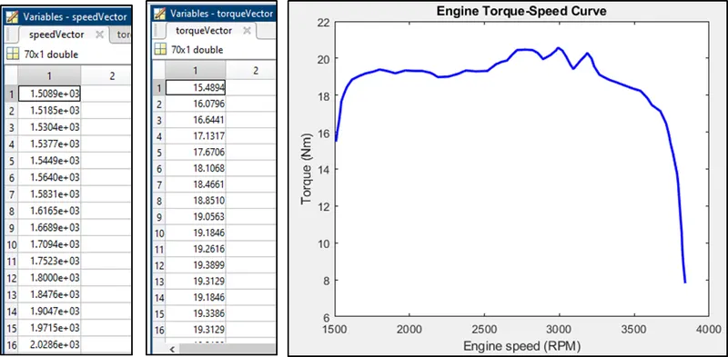
The torque and speed data required for engine is obtained and extracted and given as torquevector, speedvector variable in Base workspace.
- Engine sensor:
In this subsystem an ideal rotational motion sensor is used which measures the engine RPM. The engine RPM is then further seen by scope.
- CVT :
In this subsystem a Variable Ratio Gear block is used which represents the CVT. The two Inertia blocks are added to represent primary and secondary pulley. Further two ideal rotational motion sensors are added to measure the CVT primary and CVT secondary RPM. Rotational reference is connected to C ports.
- Simple Gear:
After CVT, simple gear box is added having gear ratio of 10 and connected to vehicle body block.
6. Vehicle Body :
In this subsystem following blocks are used
A. Vehicle body : It is used to represent the physical model of vehicle in which
Mass= 250Kg, Number of wheel per axle=2, Horizontal distance from CG to front axle= 1m, Horizontal distance from CG to rear axle= 0.35m, CG height above ground=0.7m, For drag- frontal area=0.735482m^2, drag coefficient=1.92, air density=1.18 Kg/m^3.
B. Inclination is given as 0 by PS constant block also, wind velocity is given as 0 by PS constant block.
C. Tire : 4 blocks are added to represent the physical model of tire (Front and Rear) and are connected to NR and NF port of vehicle body block.
D. Double Shoe Brake : It is used to represent the brake to which input is given from brake signal generated in signal builder with Gain of 1000. S port is connected A port which is mechanical rotational conserving port of wheel axle.
E. Ideal mechanical rotational inertia: It is used to add inertia to wheel axle.
F. Integrator : It is used to integrate speed over time to find out the distance covered.
G. PS Terminator : It is used to terminate the signal.
7. Go-To : It is used to send signals to From blocks that have the specified tag
8. From : Receive signals from the Goto block with the specified tag
9. Scope: It is used to see the signals connected.
10. Knob: It is used in dashboard to change the brake and throttle input during simulation. Its signal is connected to constant block.
11. Lookup Table : It is used to insert the values from workspace
12. TO Workspace: It is used to extract the simulation data to workspace
13. Step-It is used to provide step signals
CASE 1- BAJA ATV MODEL WITHOUT DASHBOARD
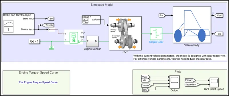
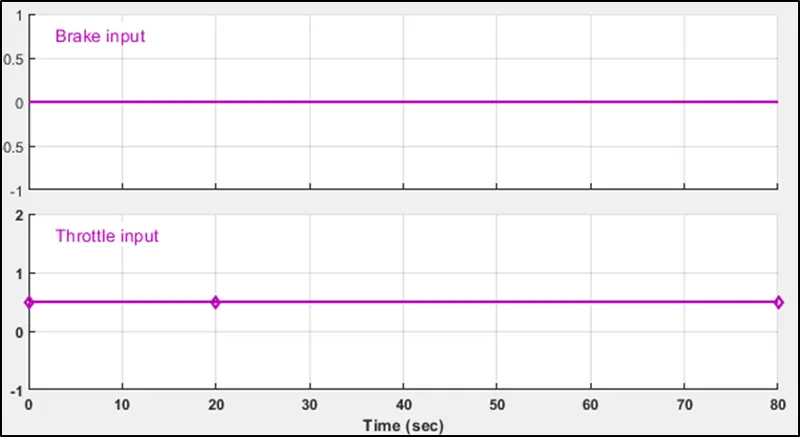
The brake signal and Throttle signal is built by signal builder. The brake is set at zero and throttle is set as 0.5 upto 80 secs.
The engine torque and speed data is given in base workspace as shown in below fig.
Throttle input is given to the engine where engine accelerates and its speed is measured by engine sensor which ideal rotational motion sensor and is seen by scope. At the end of simulation after 200 sec, the maximum engine RPM reach is 3414.76 RPM
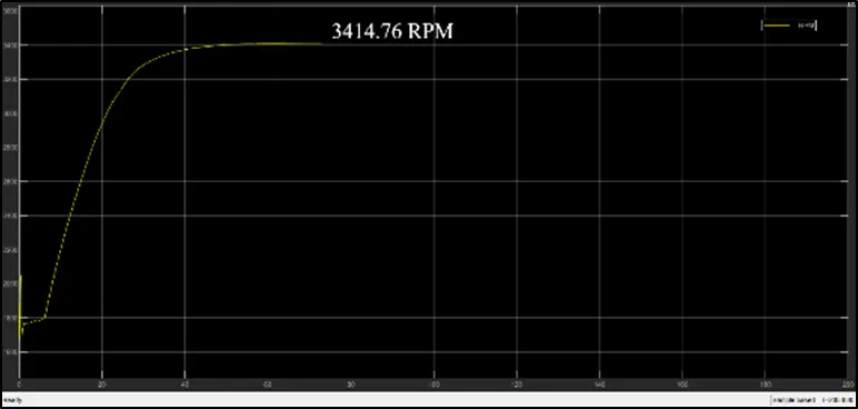
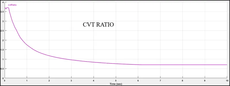
This engine speed input is given to CVT where CVT ratio is given by signal builder.
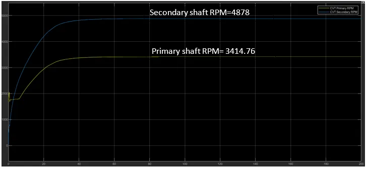
The primary and secondary shaft speed of CVT are observed as shown in below fig.
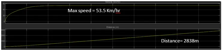
Output of CVT is given to gear box where gear ratio is 10 and increased speed is given to wheel axel. The velocity of vehicle and distance covered by vehicle are observed as shown in below fig.
CASE 2- BAJA ATV MODEL WITH DASHBOARD
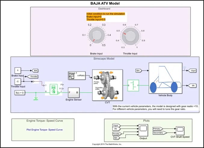
In this model the brake input and throttle input is given through the dashboard. The constant blocks are used to provide the input from dashboard. The simulation time is set at inf. To start the simulation initial condition is brake= 0 and throttle=0.5.
The connection and working of the model is same as case1. In this model we can change the throttle input and brake input while simulation and accordingly the primary, secondary shaft speed of CVT and vehicle speed changes. The observations are as shown below
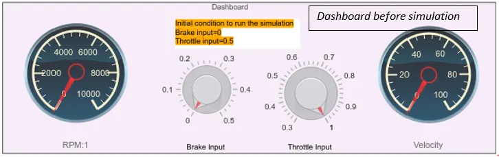
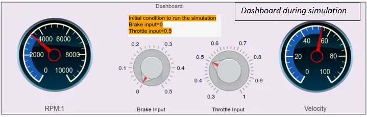
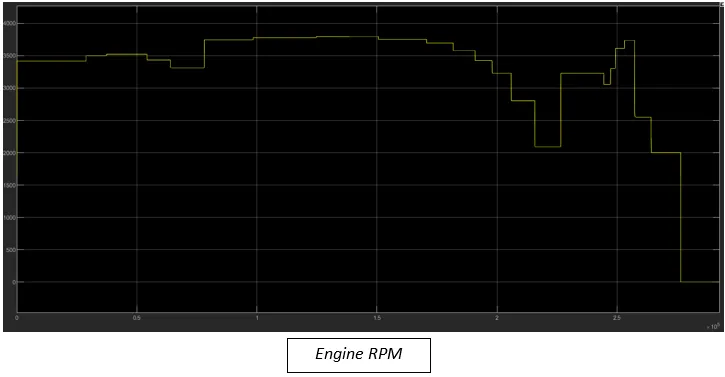
The engine RPM is generated by using speedvector , torquevector, throttle, brake input. During simulation as we change the brake and throttle knob, correspondingly the engine RPM also changes.
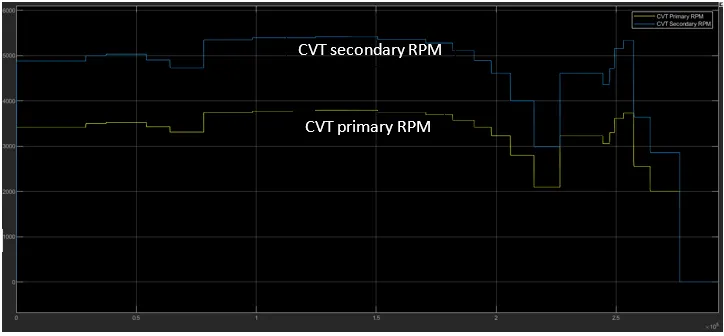
CVT primary and secondary RPM also changes as we change the throttle and brake input.
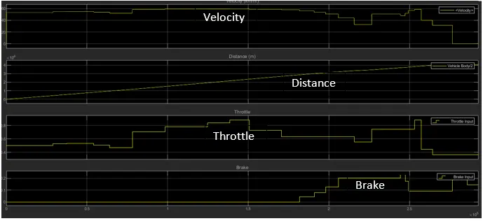
Velocity and distance changes as we change the throttle and brake input by knob.
CASE 3- BAJA ATV MODEL LOOKUP TABLE DATA EXTRACTION
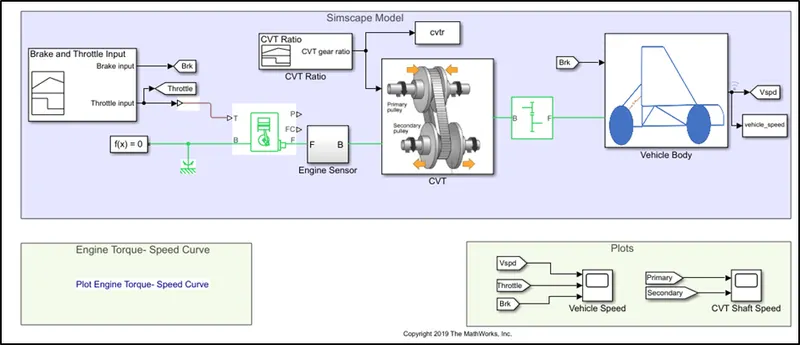
The working of the model is same as the previous cases. Here in this model the fix throttle and brake input is given by signal builder.
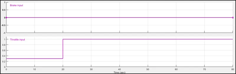
The brake =0 and throttle=0.3 initially, after 20 sec full throttle is applied which gives acceleration.
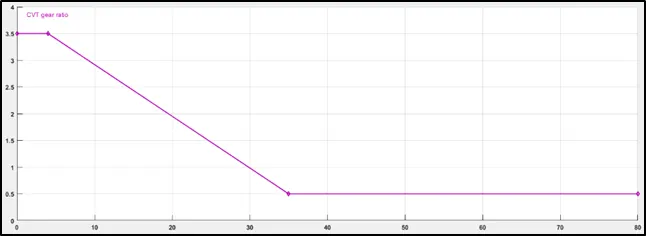
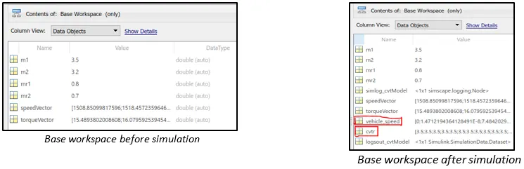
The CVT ratio is given by signal builder and then is extracted in workspace during simulation.
The vehicle speed is also extracted to workspace during simulation.
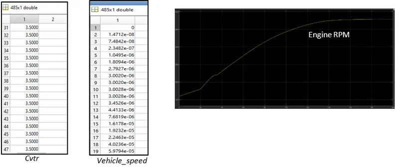
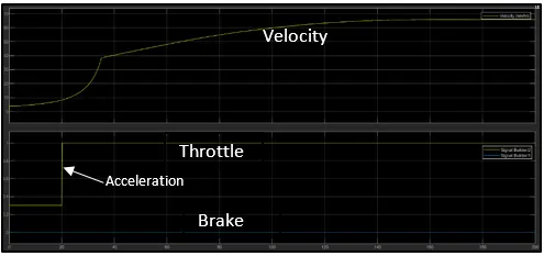
It is observed that after acceleration the velocity of vehicle increases
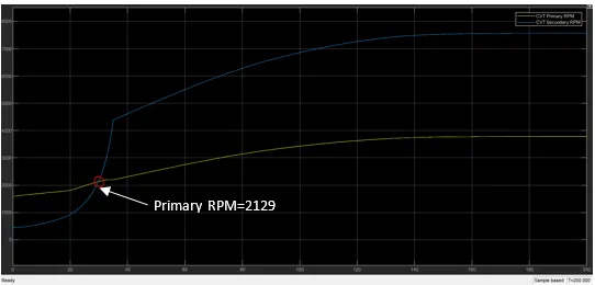
After primary RPM= 2129, CVT ration changes and become less than 1, so CVT secondary become greater than primary.
CASE4 – BAJA ATV MODEL DATA WITH LOOKUP TABLE
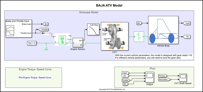
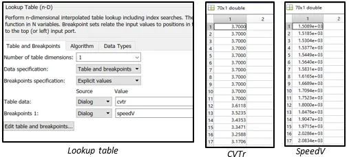
The working of this model is same as the previous cases. Here, the CVT ratio is mapped in lookup table, against the engine RPM i.e CVT ratio is selected according to engine RPM.
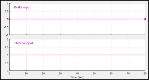
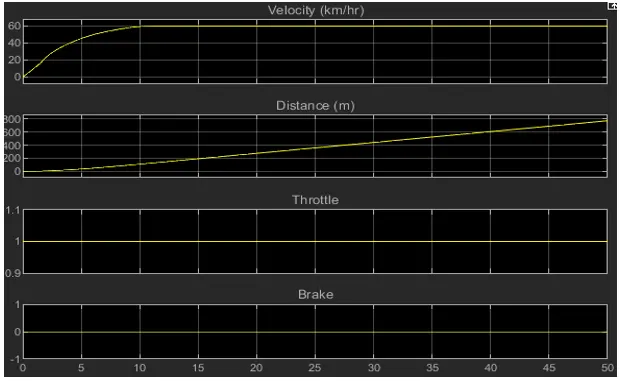
Input Brake=0, throttle=1 is given by signal builder.
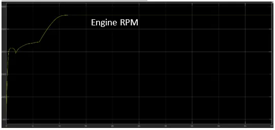
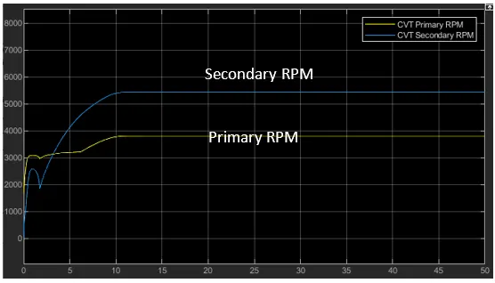
The model is simulated for 50sec. As the throttle=1 engine RPM and vehicle velocity achieved maximum speed
CASE5 – BAJA ATV MODEL MAPPED DATA WITH LOOKUP TABLE WITH DASHBOARD
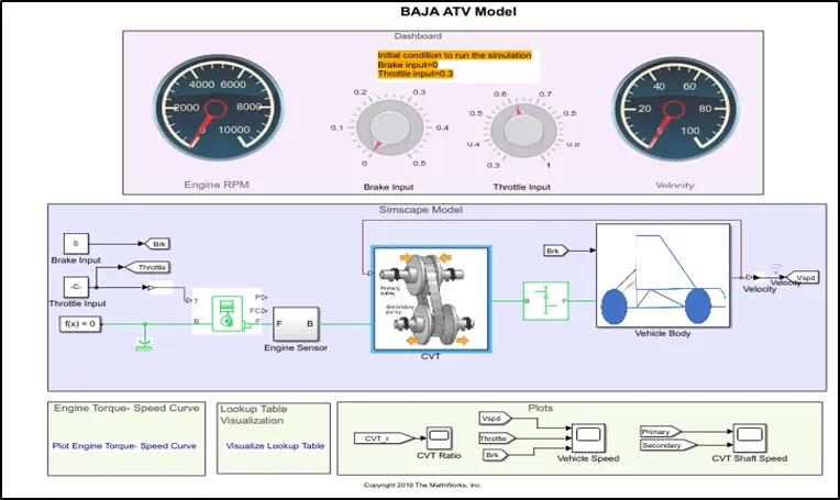
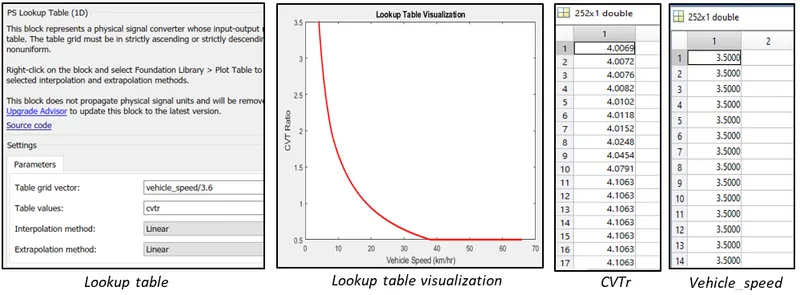
The working of this model is same as previous cases. The throttle input and brake input can be changed during simulation using knobs in dashboard. The CVT ratio is mapped in lookup table against the vehicle speed. Depending the on vehicle speed demand CVT ratio changes as per data provided in lookup table.
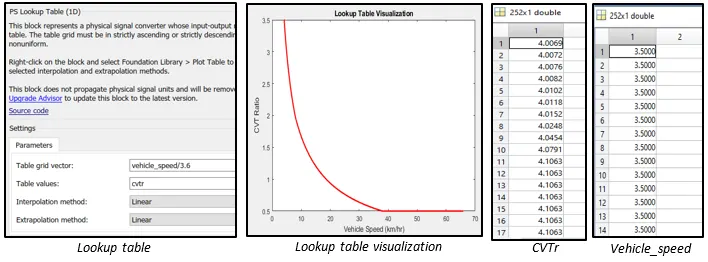
Initial condition for simulation is brake=0, throttle=0.3
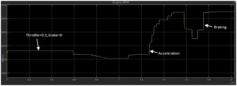
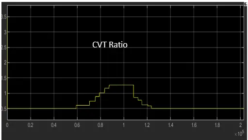
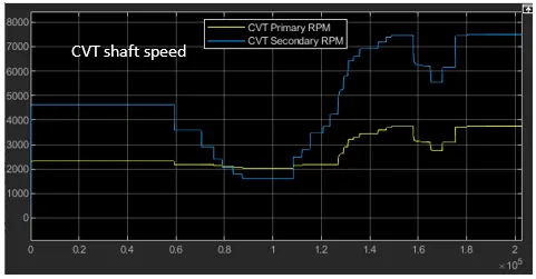
As we change the throttle and brake the CVT ratio, engine RPM, CVT shaft speeds, vehicle velocity changes accordingly. CVT ratio becomes constant at 0.5 above vehicle speed=37.9733km/hr.
CASE6- BAJA ATV MODEL MAPPED DATA WITH LOOKUP TABLE WITHOUT DASHBOARD
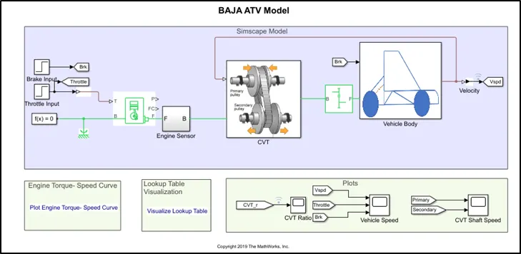
The working of this model is same as previous cases. The throttle and brake input is given by step signals. The CVT ratio is mapped in lookup table against the vehicle speed. Depending the on vehicle speed demand CVT ratio changes as per data provided in lookup table.
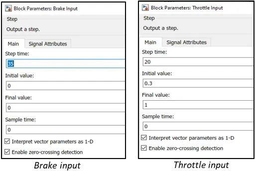
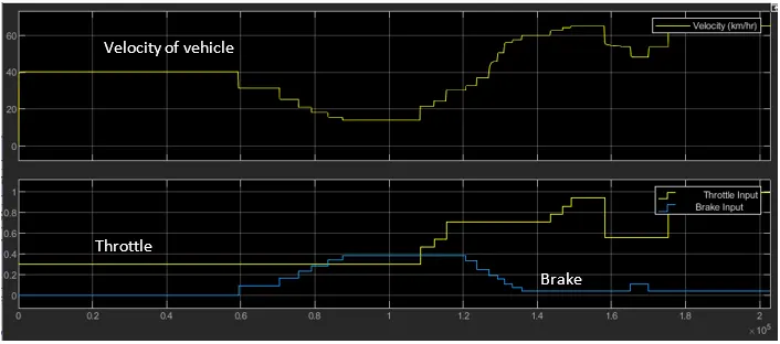
As change in throttle, brake input as per step signals, the engine RPM, cvt ratio, CVT shaft speed, velocity of vehicle changes. The simulation time is 200 sec.
As throttle input increases as per step signals, acceleration takes place and engine RPM increases, it reaches maximum constant speed after 140 sec.
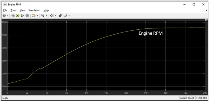
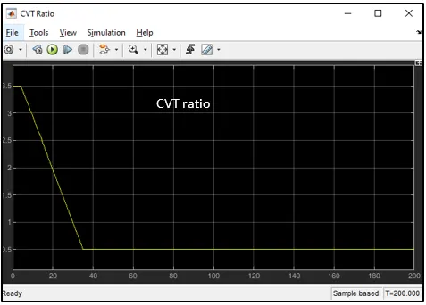
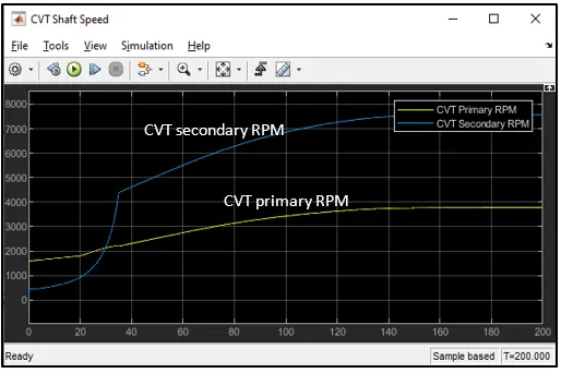
As shown in above figures, as CVT ratio changes CVT secondary RPM changes.
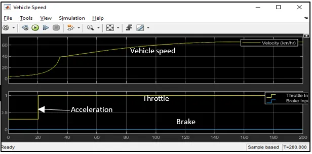
Vehicle speed increases as throttle increases and become maximum as throttle become 1.