Project

AIM -

• To Prepare a Technical Report of an All-Terrain Vehicle this has continuously variable transmission.
• We have to observe all the models and comment on each of their results.

Theory -

• We will observe six model's with different properties from each.
• BAJA ATV Model.
• BAJA ATV Model using Dashboard.
• Baja ATV Model with data stored
• BAJA ATV Model Mapped
• BAJA ATV Model Mapped with Dashboard

1. BAJA ATV -

• Let us understand what exactly an ATV is. An ATV is All-Terrain Vehicle designed to run on different types of terrain's with having low pressure tyres, mostly one-seater and could come in three-wheeler or four-wheeler as well.
• BAJA ATV is a competition where students design and fabricate their own ATV's and put it to the test.
• The ATV has to endure a lot of tests which includes agility, durability, speed, acceleration and etc.

2. CVT –
   

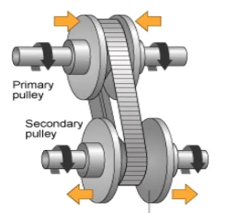
• A Continuously Variable Transmission (CVT) is an automatic transmission which can change through different gear ratios smoothly and continuously.
• A CVT allows the engine to operate at a constant RPM while the vehicle is moving with different speeds.
• Different gear ratios are achieved by continuously changing the diameter of the Pulley’s. If Primary length is increased, the Secondary length will decrease automatically and vice-versa.
• It is generally connected by a steel chain rather than a rubber chain. The Steel chain can sustain the constant force while transferring the torque from Primary Pulley to Secondary Pulley.
• There are Various Types of CVT’s, we have the Pulley-Based Type in our model. Some other types of CVT’ are Toroidal, Hydraulic, Electric etc.
• It offers a better Fuel-Economy than AMT’s
• Some of its limitation are – Maintenance is difficult, Limitations on Power, No Feeling of connectivity between the accelerator and the engine and Noise at higher speeds.

Case Study Number One -

• BAJA ATV Model
  
  

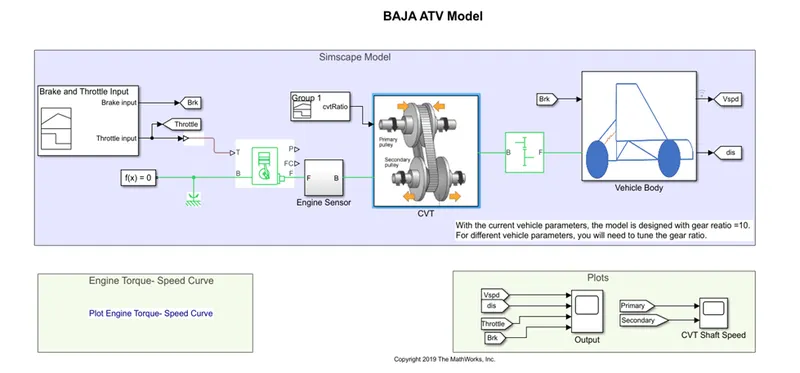
This is the BAJA ATV with CVT Simulink Model and we will further analyze every block, the mechanism and Results.

• Brake and Throttle Input -
  

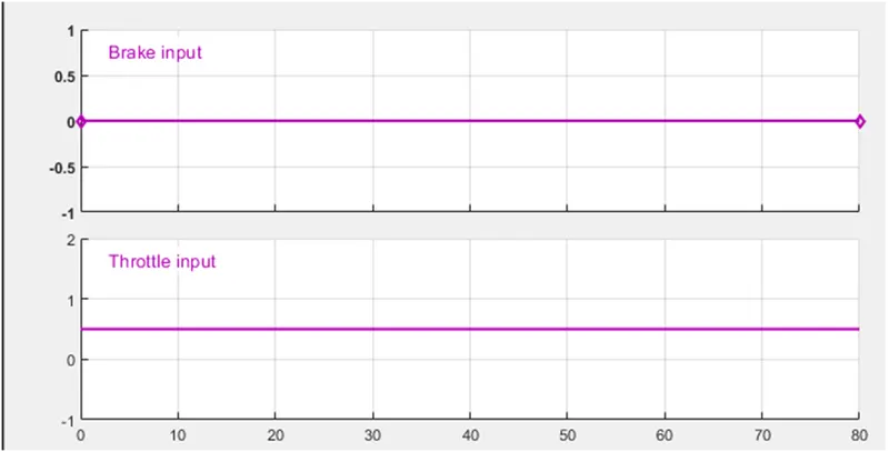
• This is a Signal Builder in which we have defined two inputs – Brake and Throttle.
• Clearly we can see that Brake Input will be 0 throughout this Simulation.
• Similarly, Throttle Input will be 0.5.

• Matlab Inputs –
  

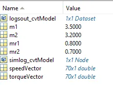
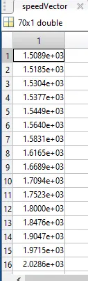
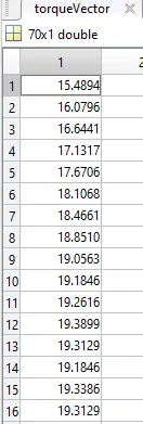
• These are Matlab Input variables which are used in the model for different blocks, we will have a better look at these inputs when we come across the blocks itself.
• We can see 6 Input variables i.e m1, m2 , mr1, mr2, SpeedVector and TorqueVector.

• Generic Engine –
  
  

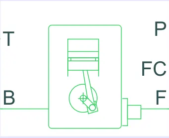
• This Block represents a general IC Engine. This is our main engine and we will further observe parameters related to this block. Speed Vector and Torque Vector values are pre-defined mentioned in the above Matlab Inputs.
• Ports – T = Input Throttle, P = Engine Power, FC = Fuel Consumption, B = Base Port, F = Engine Crankshaft (Follower).
• The B Port is connected with Mechanical Rotational Reference and Solver Configuration. The later block can be connected anywhere in the system, but it is a necessary block.
• The Throttle Input is fed to the T block of engine through Simulink-PS Converter.
• In this model, we haven’t used FC or P port.
• Now, F is the output port and it is fed to the Engine Sensor Subsystem.

• Engine Sensor –
  

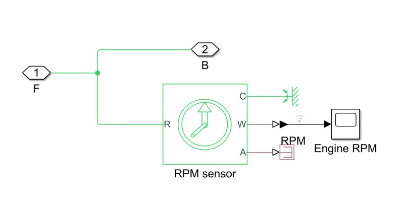
• The Engine Sensor Subsystem helps us to know the Engine RPM. The Follower of generic engine comes from 1, which is then fed to RPM Sensor and sent directly to CVT Subsystem via 2.
• Let us understand RPM Sensor in detail. There are four ports visible to us. R – Rod, C – Reference, W – Angular Velocity, A – Angular Displacement.
• A Port is terminated, C is reference, W is fed to Engine RPM Scope via PS-Simulink Converter.

• CVT Ratio –
  
  

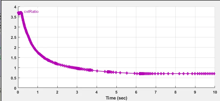
• This is the CVT Ratio Input Block. We can see 2 Inputs to the CVT Subsystem, One will be this input and other one is from Engine Sensor.
• This Input is the reason why there is going to be a change in CVT Primary RPM and CVT Secondary CVT RPM. We can clearly see that, initially the value is high and then it gradually comes down under 1.
• The Input perfectly depicts the starting condition of a vehicle, where we need higher torque at initial gears.

• CVT Subsystem –
  

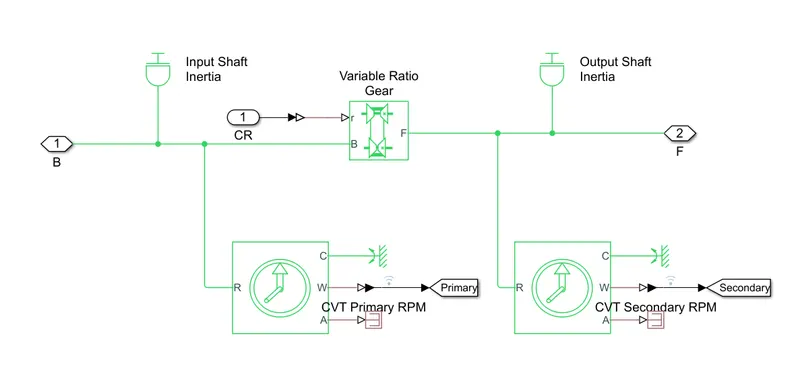
• This is Inside the CVT Subsystem, we can see Inertia comes into play when we are transferring the torque.
• There are two types of inertia present here, Input Shaft Inertia and Output Shaft Inertia. m1 and m2 are in the inputs of the inertia’s, which are inputs taken from the Matlab Inputs.
• In this subsystem, we have 2 inputs CVT Ratio which is fed to variable Gear Ratio and Follower from Generic Engine which is also fed to the Variable Gear Ratio.
• We use two RPM Sensor’s two check and compare Primary and Secondary RPM’s.
• Now, lets look at Variable Gear Ratio in deep -
  
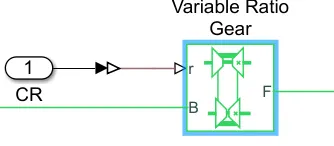
  Ports – B = Base Drive Shaft. F = Follower Drive Shaft. R = Input-to-output shaft velocity Ratio.
  The CVT Ratio Input will decide the relation between B and F. We will see in results how CVT Ratio affects the RPM later.
• Now Moving on to the subsystem, the Follower is sent to Vehicle Body via a Simple Gear which has a Gear Ratio of 10.

• Vehicle Body Subsytem -

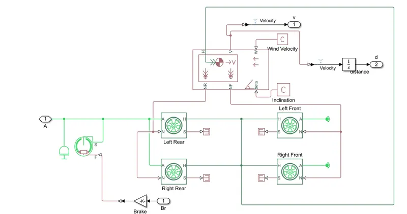
• In this Subsystem, we will have 2 Inputs and 2 Outputs. Brake and A From Simple Gear are Inputs while Velocity and Distance are the outputs.
• Brake is fed directly from the 1^st Signal Block we discussed earlier, It is multiplied by 1000 using a Gain block. As we have brake Input = 0, we wont look into Double-Shoe Brake in detail.
• We have Vehicle Body and 4 tyres connected with each other.

• Tyres –

• Ports – A = Axle, N = Normal Force, H = Hub, S = Slip. We can see that S block is terminated from each tyre.
• The Torque coming from the Simple Gear is fed to Rear Wheels through A port. A Port of Front wheels have a rotational free end as the power is fed to Rear Wheels and Front wheels are used to give the direction to the vehicle.
• The H Port of all tyres are connected to the H Port of of vehicle body, which gives us the horizontal motion of the vehicle.

• Vehicle Body –

• This block represents a two-axle Vehicle Body in which we can choose Wheels per axle, Mass, Drag, Pitch etc.
• Ports – V = Velocity, H = Horizontal Motion, NR = Rear Axle Normal Force, NF – Front Axle Normal Force, There are other ports as well but the effect of them in this model is negligible.
• The Output Velocity is directly given to the scope, which we will study later on. Further, the velocity is integrated which turns it to Distance and it is given as a second output.
• NR and NF are connected properly as we can see in the above Vehicle Body Subsystem.

• Results –
  

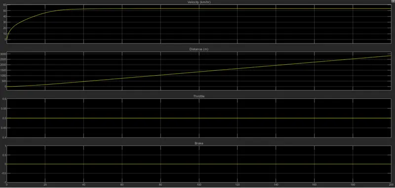
• These are the results from Output Scope which shows us Velocity, Distance, Throttle and Brake.
• As we have discussed earlier, Brake and Throttle are ngoing to remain same throughtout the simulation, which is evident in the results.
• Now, the Distance is constantly increasing w.r.t time at nearly a constant rate.
• Looking at the Velocity Parameter, we can observe that after initial rise the velocity remains constant. This is because we haven’t applied brakes or increased throttle input and the gear ratio remains same after initial change.
  
  
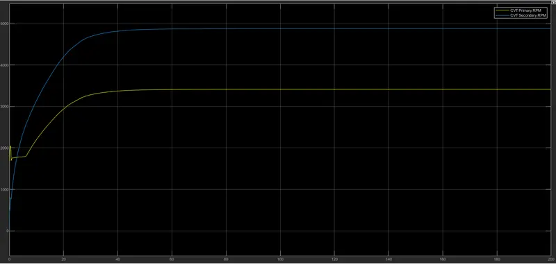
• CVT’s main aim is to keep the RPM Constant for various speed’s. From this Result we can observe that RPM’s are pretty constant.
• The Initial difference in RPM’s is due to the Gear Ratio Input. We have note that Engine RPM = CVT Primary RPM.
• Initially Primary RPM is greater than Secondary RPM just for few seconds, i.e To start the vehicle we need High torque.
• There is a point at which both the RPM’s meet, that point is where the Gear Ratio = 1.
• After that point, Secondary RPM becomes greater than Primary. This means the Secondary Pulley will get more revolutions which will be reflected on the tyres of the Vehicle.
• Both the RPM’s remain constant after that.

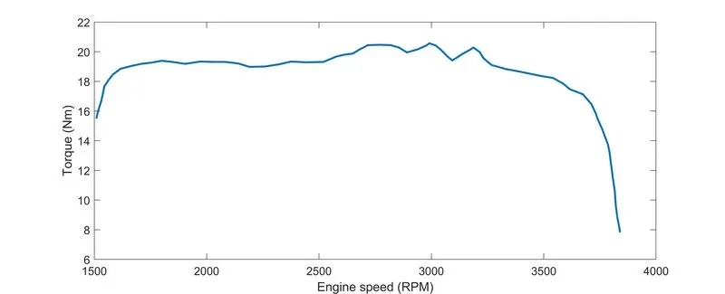
• This plot is between Torque and Engine RPM. Torque values are already given to us from MATLAB inputs.
• From the above plot we can clearly see that Engine RPM reaches a maximum level of 3840 and during the initial stage it is 1509.
• Further we can also observe that Maximum Torque value is 20.57 and it reaches 7.817 in the end.
• From the above values and observations, we can clearly comment that Torque required in the initial stage is high and then after some time it gradually decreases to the lowest level in this case. But, the RPM keeps on rising till the 3840 level and is constant after that.

Case Study Number Two -

• BAJA ATV Model using Dashboard

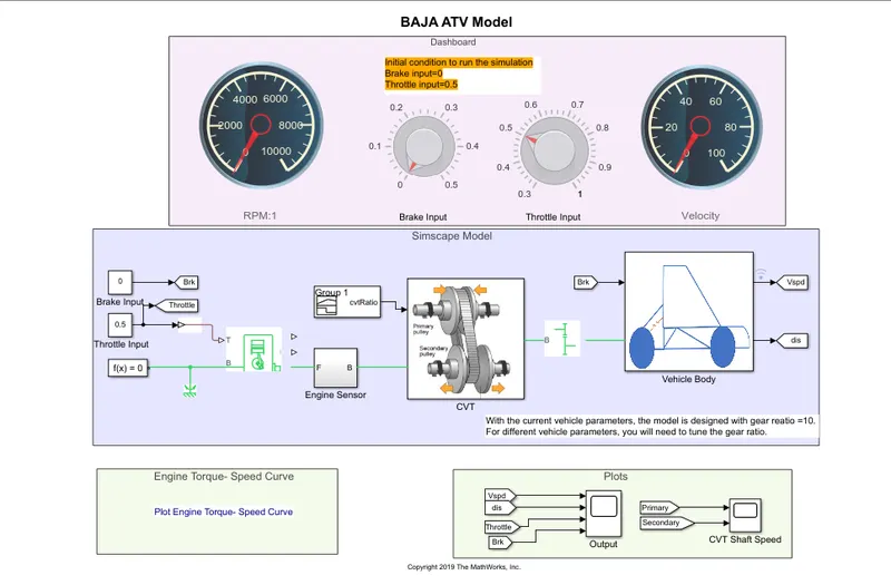
• This is Simulink Model for BAJA ATV with CVT and Dashboard. Dashboard is provided to change the Input values and observe the effects immediately
• There is not much difference between the previous model and this model. The only difference is Dashboard, which has two Knobs and two Gauges.
• The two Knobs are connected with Throttle input and Brake Input. We can vary these inputs while the simulation is running.
• The Two Gauges will show us the Engine RPM and Velocity.
• The Simulation time is kept as infinite as we will keep changing the input values as the simulation goes on.
  
• The Initial Condition given to us is Brake Input = 0 and Throttle Input = 0.5.
  
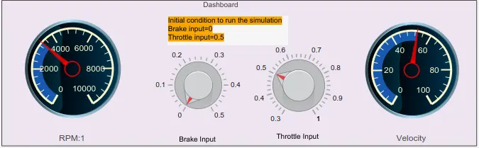
• The Dashboard reflects the initial condition and shows us the Speed and RPM after settling down. Both RPM and Velocity will increase gradually the above values. Now we will look at the dashboard when we change the Input Values -
  
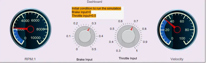
• Now, we can clearly see how Brake will impact the Engine RPM and velocity. In this case Brake Input was kept 0.3 and Throttle was slightly increased to 0.7.
• Now let's move on to the Final Results and observe them.
  

• Results -
  

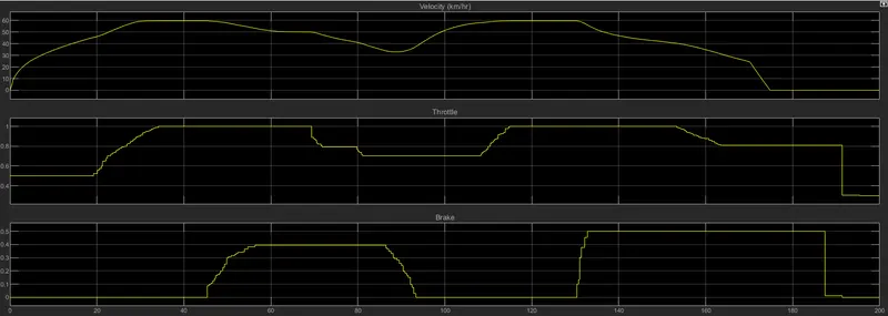
• In this Scope Result, we will analyse how Velocity changes with respect to Throttle Input and Brake Input. These results are obtained by changing the simulation pacing and time for proper scope results, so we can analyse them.
• We can Observe that Velocity increases as the Throttle Input is also increased and Brake Input is kept at 0.
• As soon as we apply brakes, the velocity comes down suddenly. Then again, brakes are down to low level and Throttle Input is increased.
• We can observe that Velocity will climb to it's peak value again as both the Inputs are in favour.
• At last, when we apply maximum brakes the velocity becomes 0. That is because of Generic Engine we studied earlier, If the engine speed goes below the 'Stall Speed' the torque will blend to zero.
• Thus, we can see the velocity will remain 0 even if we change the Inputs in the favour of velocity.

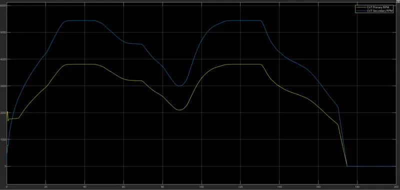
• These are results obtained from CVT Shaft Speed Scope.
• The CVT Primary RPM is the RPM we observe on the Dashboard. The same initial condition is observed in this model as well, then Secondary RPM will rise and then will be related to the Primary RPM in a constant manner as we do not change the Gear Ratio.
• Further, we can observe how RPM's respond to the Throttle and Brake Inputs.
• At the end of the simulation we observe torque as zero, it is very well reflected on the RPM's as well. Both the RPM's come down to zero.

Case Study Number Three -

• BAJA ATV Model with using Lookup Table

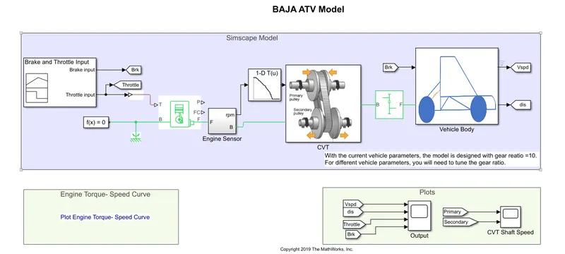
• This is the Simulink Model for BAJA ATV using Lookup Table. Here, instead of Signal Builder Block of CVT Ratio, we will use a 1-D Lookup Table for the data.
• There is not a much of a difference between this model and first model we studied, Only Lookup table and few minor changes are present in this model which we are going have a look now.

• Brake and Throttle Input -

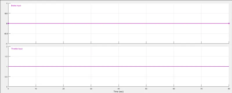
• These are going to be our Brake and Throttle inputs for the whole simulation.
• Brake Input is 0 and Throttle Input is 1.

• Matlab Inputs -
  

• These are cvtr and SpeedV data/inputs which are already defined in the MATLAB.
• We can see these variables inside Lookup Table, which we will study later.
• cvtr is table data which will be reflected as output from the Lookup Table and SpeedV data are the Breakpoints provided as an input.

• Lookup Table -
  

• We use a Lookup table for the CVT Ratio Input in this model. Lookup table will map input values to a certain output value, which is in form of a table.
• Here, we will be obtaining output as cvtr which will be dependant on the imput value i.e SpeedV.
  
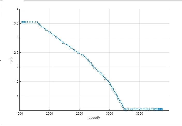
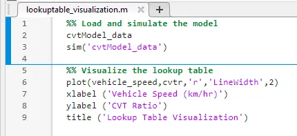
• Above image shows us which cvtr value will be given for which SpeedV value. We have to note that SpeedV is the Engine RPM. There are total 70 values of both variables which can be seen in MATLAB or in the Lookup Table itself.
• Now, we will look at the Lookup Table Code, which will make things much more clear.

• Results -

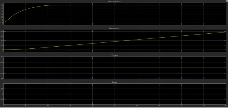
• These are the Scope Results Obatained after Simulation is carried out.
• We can observe that Brake and Throttle inputs are constant throughout the Simulation.
• Distance will keep increasing as we do not apply brakes and Throttle is constant as well.
• Velocity will keep increasing till 60km/hr and will remain constant because we do not change Gear Ratio or Throttle Input in this Simulation

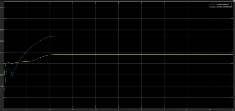
• These are CVT Scope Results to analyse and compare CVT Primary RPM and CVT Secondary RPM.
• We can observe that, only initially Primary RPM is greater than Secondary RPM. This is due to high Gear Ratio and Torque which is required to start any vehicle.
• After a certain time, the Gear Ratio becomes constant and them RPM's will remain constant as well.
• Secondary RPM is greater than Primary RPM because of Gear Ratio being lower than 1.

Case Study Number Four -

• BAJA ATV Model with Data Stored

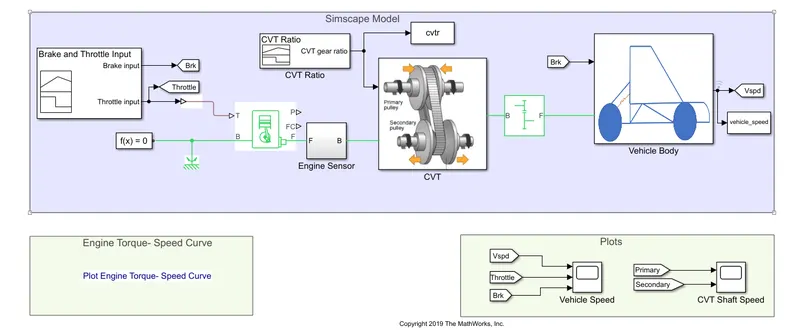
• In this Model, we can see that CVT Ratio and Vehicle Speed are being stored to Matlab using The 'To Workspace' Block.
• Let's have a look at the Brake and Throttle Inputs -
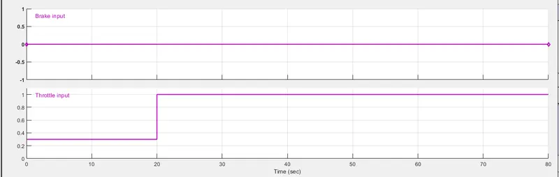
• Throttle Input is like a step input, which will step-up at 20 seconds. Meanwhile Brake Input will remain 0.
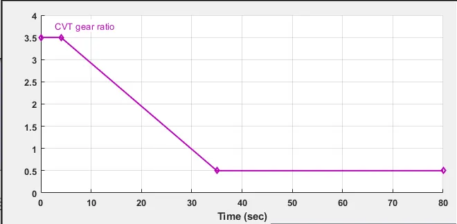
• Now let's look at CVT Ratio for this model -

• Results -

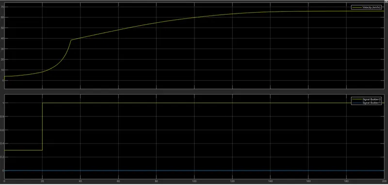
• These are scope results which show Vehicle Speed, Brake and Throttle Input.
• As we can see, there is a sharp rise in vehicle speed after Throttle Input is tepped up.

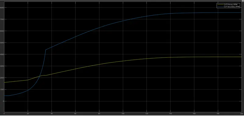
• This is CVT RPM Comparison Scope Results.
• As, the CVT Ratio changes and Throttle Input is changed we can see that Secondary RPM becomes greater than Primary RPM. As the CVT Ratio becomes 0.5 and remains constant, we can see good amount of difference between the RPM's.

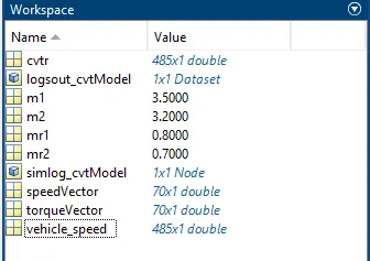
• After the Simulation, we can check the CVT Ratio and Vehicle Speed in Matlab.
• cvtr and vehicle_speed will show us the values of CVT Ratio and Vehicle Speed respectively.

Case Study Number Five -

• BAJA ATV Model Mapped
  
  

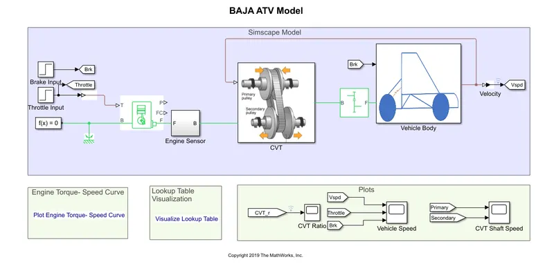
• This Model is BAJA ATV Mapped Model. Here, we can see the CVT Ratio is dependant on the Vehicle Velocity.
• Previously, we saw that CVT Ratio was eirther given by Signal Builder Block or was linked with Engine RPM.
• In this model we have used PS Lookup Table(1D), which has Physical Signal as an input and output.
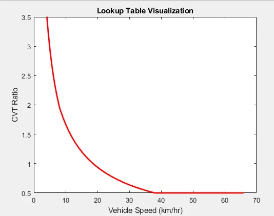
• Above image is the Lookup Table Visualisation, gives the idea of how CVT Ratio will vary with respect to Velocity of the Vehicle.

• Results -

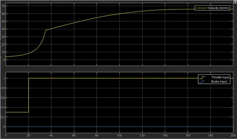
• These are the Scope Results in which we will analyse Brake, Throttle and Velocity.
• Brake is zero for whole Simulation.
• Throttle Input is a Step Input which jumps from 0.3 to 1 at 20 Seconds.
• After the jump, the same is refelcted in Velocity as it incrases rapidly after 20s. Then Velocity is increased gradually because on the change in CVT Ratio.

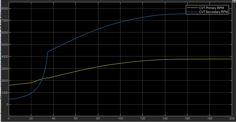
• Now we compare the CVT Primary and CVT Secondary RPM's. There is nothing worth noting in this Result as it is similar to the previous Results.
• Initially the Primary CVT is greater and after CVT Ratio goes below 1, Secondary CVT RPM becomes greater.

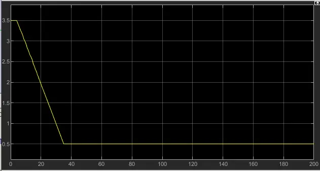
• This CVT Ratio Result will show us how CVT Ratio varies with respect to time.
• Initially, it is 3.5 which then slowly comes down to 0.5.
• After watching this result we can have a clear idea of why Velocity reacts after the CVT Ratio becomes 0.5.

Case Study Number Six -

• BAJA ATV Model Mapped with Dashboard

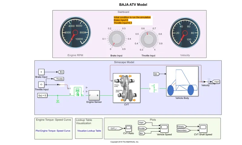
• This is how the Model looks with a Dashboard. We can change Brake and Throttle Inputs while the Simulation is running.
• It is Similar to the previous Model where we used a PS Lookup Table and the Input was Velocity of the Vehicle. Velocity and CVT Ratio were related, now we check their co-relation even better in this model.
• Let's have a clear look at the Dashboard -
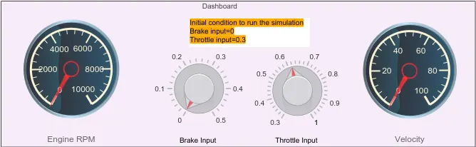
• In Dashboard we have two Knobs and two Gauges. Knobs will help us to change the Input values and Gauges will display Engine RPM and Velocity of the vehicle. Initial Condition is given in the Dashboard itself.
• As we have Mapped CVT Ratio with Velocity, we will see change in CVT Ratio wrt Velocity. In all previous model's CVT Ratio was constant after a certain time.
  
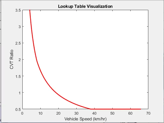
• This is how CVT Ratio will change with respect to velocity. Let's look at the results as we perform the Simulation.

• Results -

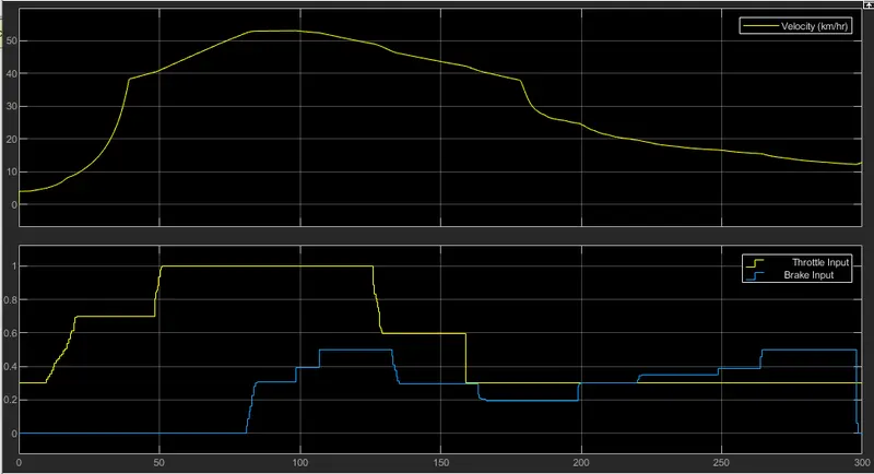
• These Results are taken after slowing down the Simulation Pacing and limiting the Simulation to 300 seconds. This is done to obtain better results and proper Scope Results for Analysis.
• Now, the above results will show us Velocity, Throttle Input and Brake Input.
• As we can see that increasing throttle increases the velocity and Similarly decreasing throttle decreases Velocity.
• Initially we do noy apply brakes at all, then we slowly incrase Brake Input to bring down the velocity.

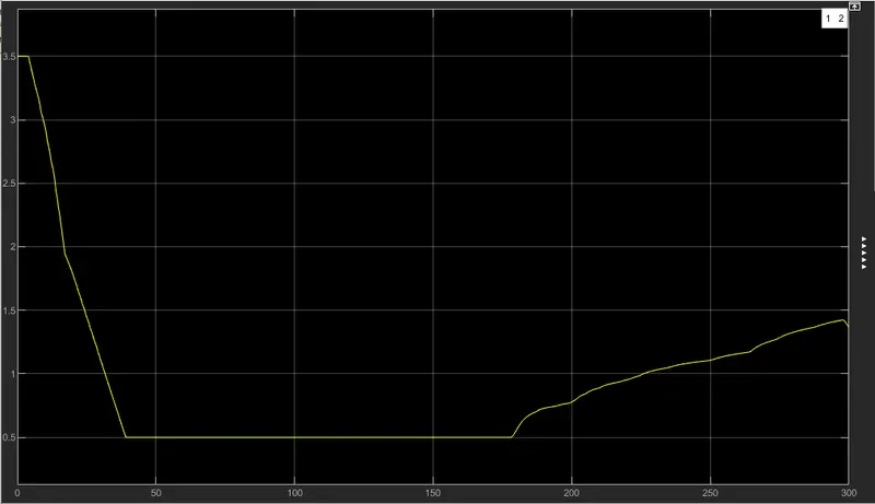
• The above results shows us how CVT Ratio will vary wrt time.
• It acts noramlly till 180 seconds, as the velocity has not dropped significantly till then.
• After that, we can see increase in CVT Ratio as Velocity drops below 38km/hr. We can Refer the Lookup Table Visualization on why does CVT Ratio increases.
• As the velocity keeps decreasing the CVT Ratio keeps increasing, After a point it even goes above 1 which will have a impact on RPM's.

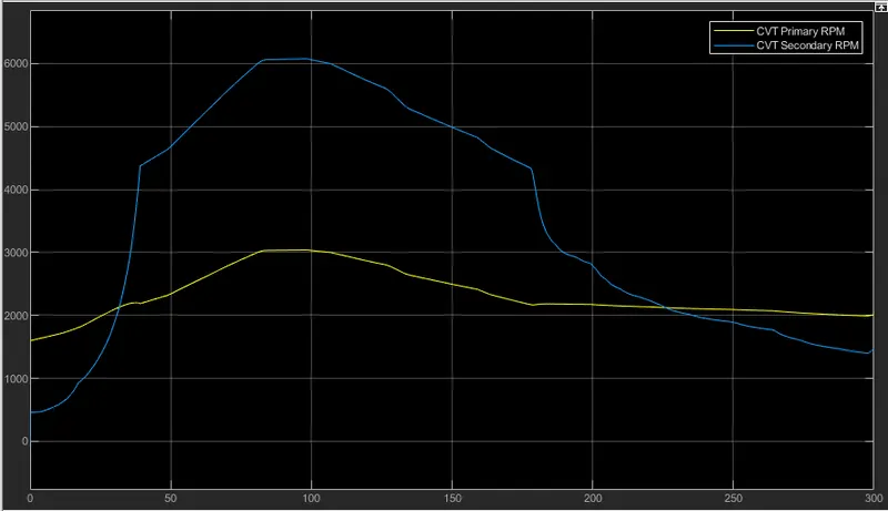
• Above is CVT Scope Result.
• We can see that as CVT Ratio lowers down below 1, Secondary RPM gets greater than Primary RPM. This Condition we have been witnessing in all previous models.
• Now, as the Velocity drops and CVT Ratio increases, we can observe that the difference between CVT RPM's gets lesser and lesser.
• Eventually as the CVT Ratio goes beyond 1, the Primary RPM(Engine RPM) will be greater than Secondary RPM.

CONCLUSION -

• Hence all the model's are observed and a technical report has been created on model property and their results.
• Basic Constrction and Blocks have been explained in the first model and any new blocks introduced have been explained as per requirement.