Project
AIM-
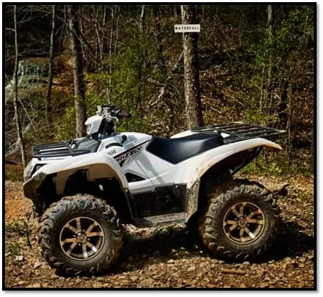
To prepare a technical report explaining the BAJA All-Terrain Vehicle (ATV) model with Continuously Variable Transmission (CVT)
Theory-
Continuous Variable Transmission (CVT)-
A continuously variable transmission (CVT) is an automatic transmission that can change seamlessly through a continuous range of gear ratios. This contrasts with other transmissions that provide a limited number of gear ratios in fixed steps. The flexibility of a CVT with suitable control may allow the engine to operate at a constant RPM while the vehicle moves at varying speeds. CVTs are used in automobiles, tractors, motor scooters, snowmobiles, bicycles, and earthmoving equipment.
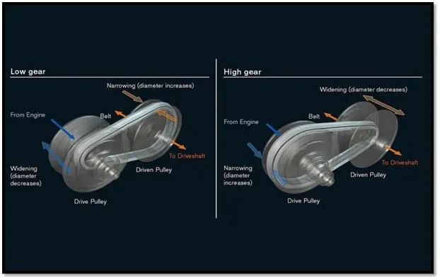
The most common type of CVT uses a V-belt which runs between two variable-diameter pulleys. The pulleys consist of two cone-shaped halves that move together and apart. The V-belt runs between these two halves, so the effective diameter of the pulley is dependent on the distance between the two halves of the pulley. The V-shaped cross-section of the belt causes it to ride higher on one pulley and lower on the other; therefore, the gear ratio is adjusted by moving the two sheaves of one pulley closer together and the two sheaves of the other pulley farther apart.
Objective-
- To carry out a system-level simulation of an all-terrain vehicle
- Understand the working of the model and analyze the results
- Prepare a detailed report
Body content-
BAJA ATV model with Continuously Variable Transmission (CVT) consists of the following Simulink blocks:
- Signal builder: The Signal Builder block allows you to create Signal sources and use them in a model.
- Go to: The Goto block passes the signal to the Form block without being connected.
- Simulink-PS converter: Converts Simulink signal to a Physical signal.
- PS-Simulink converter: Converts the input Physical Signal to a Simulink output signal.
- Solver configuration: Defines Solver settings to use for Simulation.
- Mechanical Rotational reference: This block represents a mechanical rotational reference point, that is, a frame or aground. It is used to connect mechanical rotational ports that are rigidly affixed to the frame (ground).
- Generic Engine: Represents a system-level model of spark-ignition and diesel engines suitable for use at the initial stages of modelling when only the basic parameters are available.
- Ideal Rotational Motion Sensor: This block measures angular velocity or angle in a mechanical rotational network. The sensor is ideal since it does not account for inertia, friction, delays, energy consumption, and so on.
- PS Terminator: Use this block to terminate physical signal outputs.
- Scope: Display signals generated during Simulation.
- Inertia: The block represents an ideal mechanical rotational inertia.
- Variable Ratio Transmission: Represents a variable ratio gearbox such as implemented by mechanical belt CVT, electric, or hydraulic transmissions. The physical signal input r defines the ratio of input to output angular shaft velocities.
- Simple Gear: Represents a fixed ratio gear or gearbox.
- Double Shoe Brake: Represents a brake arranged as two pivoted rigid shoes symmetrically installed inside or outside a drum and operated by one actuator. The actuator force causes the shoes to exert friction torque on a shaft connected to the drum.
- Gain: Element-wise gain (y = K.*u) or matrix gain (y = K*u or y = u*K).
- Tyre: Represents the longitudinal behaviour of a highway tire characterized by the tire Magic Formula. The block is built from Tire-Road Interaction (Magic Formula) and Simscape Foundation Library Wheel and Axle blocks. Optionally, the effects of tire inertia, stiffness, and damping can be included.
- Vehicle Body: Represents a two-axle vehicle body in longitudinal motion. The block accounts for body mass, aerodynamic drag, road incline, and weight distribution between axles due to acceleration and road profile. The vehicle can have the same or a different number of wheels on each axle. Optionally include pitch and suspension dynamics or additional variable mass and inertia. The vehicle does not move vertically relative to the ground.
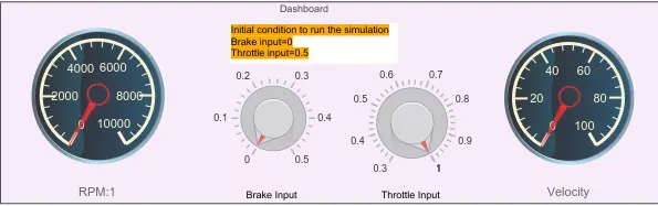
Dashboard blocks-
The below figure shows the Dashboard blocks used in the model for signal input and observing output.
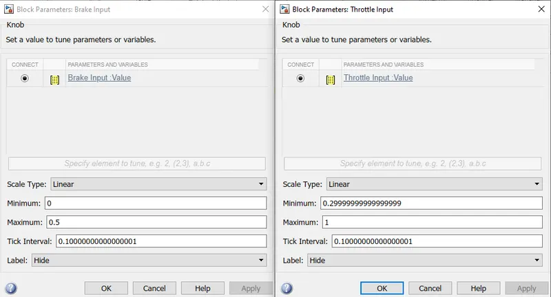
- Knobs are used for Brake input and Throttle input. The below figure shows the Knob block parameters for Brake input and Throttle input. Minimum and Maximum parameters for Brake input are set to 0 and 0.5 respectively. Minimum and Maximum parameters for Throttle input are set to 0.3 and 1 respectively.
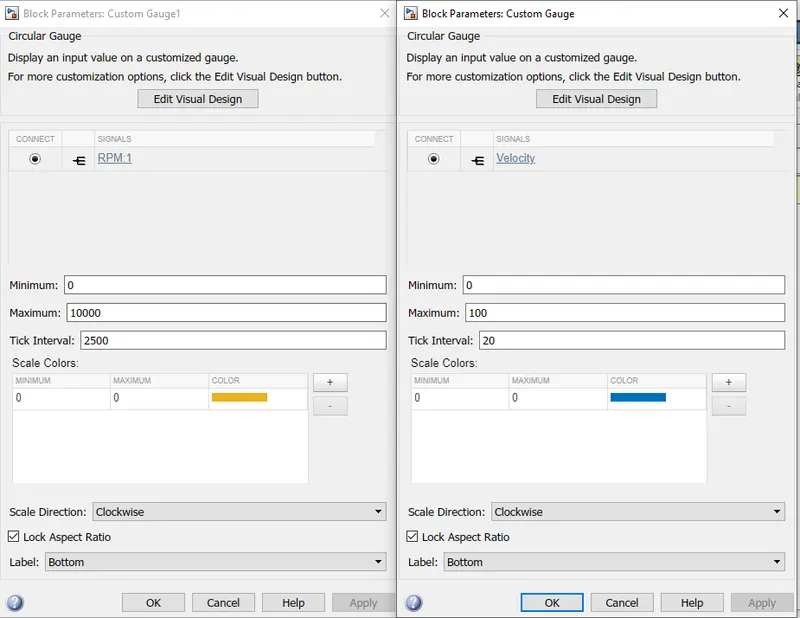
- Circular Gauges are used for observing RPM and Velocity. The below figure shows the Circular Gauge block parameters. Minimum and Maximum parameters are set to 0 and 10000 respectively for the RPM gauge. Minimum and Maximum parameters are set to 0 and 100 respectively for the Velocity gauge.
Model Subsystem-
Engine sensor-
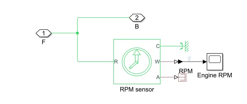
This subsystem consists of Ideal Rotational Motion Sensor Block named an RPM sensor, which has two input signal ports and two physical signal ports. Input Signal Port R is connected to the F port of the Generic Engine which is the Engine Crank Shaft and Port C is connected to a Mechanical Rotational Reference, and Physical Signal port W is connected to a Scope using a PS-Simulink Converter while port A is connected to PS Terminator. Port W gives the Angular Velocity, which is observed through Scope.
CVT-
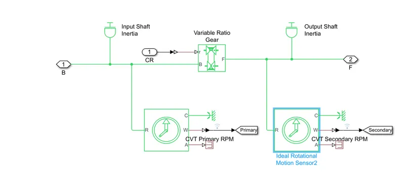
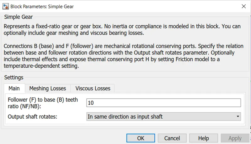
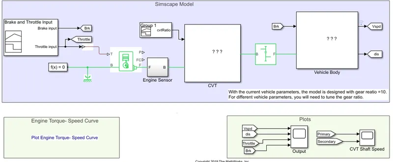
To Implement the CVT, a Variable Ratio Gear block is used with two Inertia blocks each for Input and Output shafts respectively. Variable Ratio Gear changes gear ratio according to the CVT ratio input through port r and the angular velocity from port B. This CVT ratio is created using the Signal Builder block. Two Ideal Rotational Motion Sensor Blocks are used to observe Angular velocity from the Input and Output shaft, the output signals are logged to observe using scope outside the subsystem. To Connect CVT to Vehicle Body, the speed reduction is required, so the output shaft is connected to a Simple Gear block with a gear ratio of 10.
Continuously Variable Transmission drive (CVT)
It is better to have more gears in transmission since it can optimize engine speed in a variety of driving conditions. That means low gears can provide better acceleration while higher gears can maximize fuel economy. CVTs differ from traditional automatic transmissions in that they don't have gears that provide "steps" between low- and high-speed operations. Instead, the majority of them work via a pair of variable-diameter, cone-shaped pulleys connected by a steel or composite belt. The halves of each pulley are aligned with the pointed ends of the cones touching. These form a V-shaped groove in which the connecting belt rides. One side of the pulley is fixed, and the other side is movable, actuated by a hydraulic cylinder. The cylinder can increase or decrease the amount of space between the two sides of the pulley. This allows the belt to ride lower or higher along the walls of the pulley, depending on driving conditions, thereby changing the "gear" ratio.
Vehicle Body-
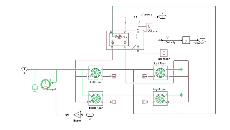
Vehicle Body Subsystem consists of a Double Shoe Brake block, Gain block, four Tyre blocks, Vehicle Body block, Two PS Constant blocks as an input source for Inclination and Wind Velocity. The output from the Simple Gear is given as input to the wheel axle A ports of Vehicle Wheels. A Double shoe brake is connected to this signal to apply friction torque when speed reduction is required. Port H in the Vehicle body block is the mechanical translational conserving port associated with the horizontal motion of the vehicle body, connected to mechanical translational conserving port H of the wheel hub through which the thrust developed by the tire is applied to the vehicle. Physical signal output ports NR and NF which are Front and Rear Normal wheel forces are connected to Wheel Axle port N, which is a physical signal input port that applies the normal force acting on the tyre. Physical signal output port V gives vehicle velocity. Connections W and beta are physical signal input ports and are connected to PS Constant blocks which are sources of Wind velocity and Inclination.
MODEL WORKFLOW-
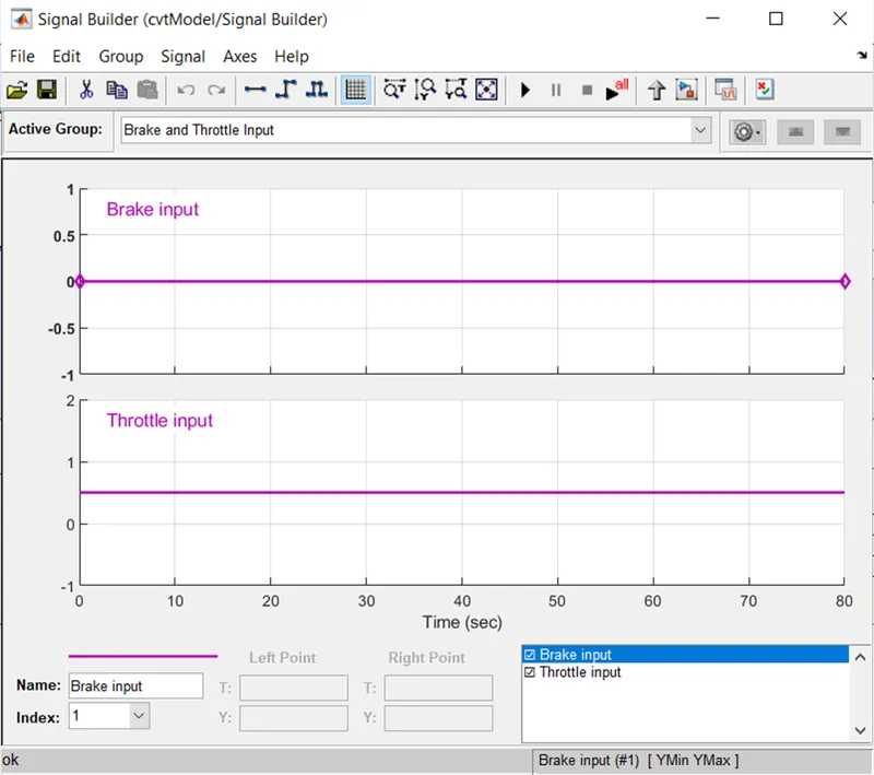
- Signal Builder block is used to generate Brake and Throttle input signal for Generic Engine. Brake and Throttle signals are logged to the scope block for observation. The below figure shows the Signal builder block with Brake and Throttle signal
- Solver Configuration and Mechanical Rotational Reference blocks are connected to Engine Block’s B port. The below figure shows Generic Engine block parameters
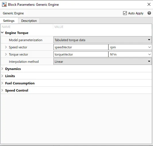
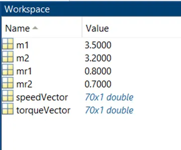
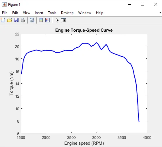
- Engine Torque parameters, ‘Speed vector’ and ‘Torque vector’ are assigned with variable inputs ‘speed vector’ and ‘torque vector’, which are defined in the base workspace. All other parameter values are used by default. The below figure shows the variables defined in Base Workspace
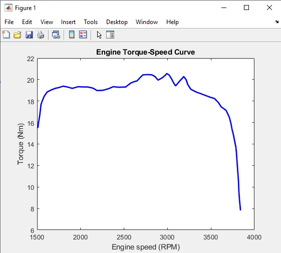
The ‘Speed vector’ and ‘Torque vector’ data are extracted from the below-shown plot
- A Subsystem named Engine Sensor is connected to the F port, which is associated with the engine crankshaft, to measure the Angular Velocity from crankshaft input.
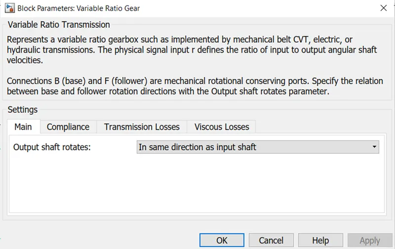
- The B port of the Engine Sensor block is connected to the Variable Gear Ratio block, which implements the mechanical belt CVT. The below figure shows the Variable Gear Ratio block parameters, where the parameter ‘Output shaft rotates’ is chosen as ‘In the same direction as input shaft’.
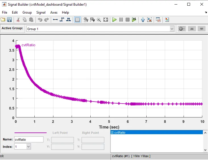
- The physical signal input r is connected to a Signal builder block, which is used as a source for the CVT ratio. The below figure shows the Signal Builder block containing the CVT ratio
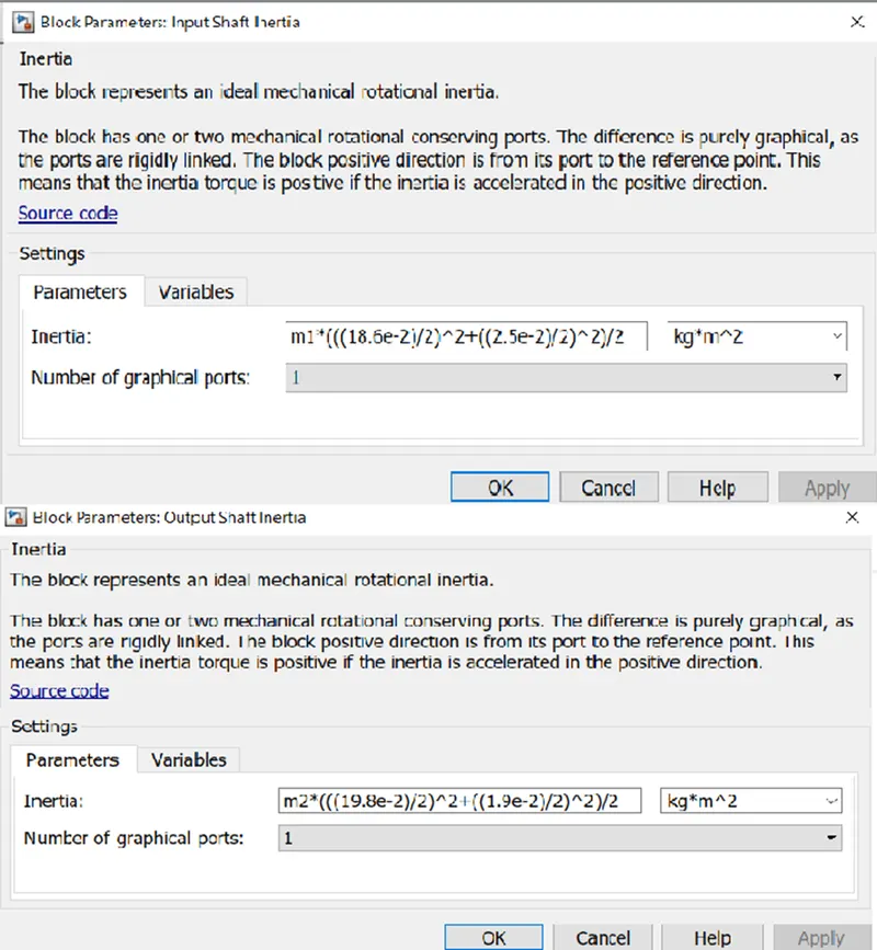
- Connections B(base) and F(follower) are mechanical rotational conserving ports and are connected to two Inertia blocks representing the Input and Output shaft. Below figures show the Inertia block parameters of the Input shaft and Output shaft, where variables m1 and m2 are defined inside the base workspace
- Two Ideal Rotational Motion Sensors are connected at the Input and Output shaft to observe the velocities at each shaft
- The output shaft is connected to a Simple Gear block with a gear ratio of 10 for obtaining speed reduction to connect the CVT to the Vehicle Body. The below figure shows the Simple Gear block parameters
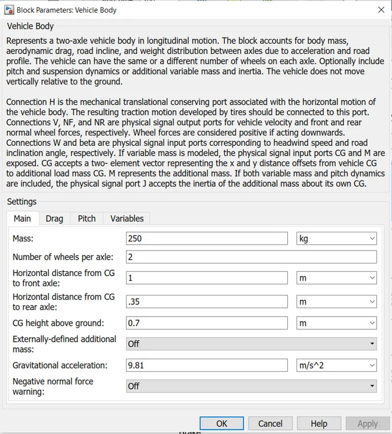
- Output from the Simple Gear is connected to the Rear Left and Rear Right Tire Block’s A port which is a mechanical rotational conserving port for the wheel axel. The H ports of all four blocks are connected to the H port of the Vehicle body block. The below figure shows the Vehicle Body block parameters
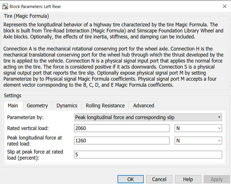
- The h port of the Tire block is a mechanical translational conserving port for the wheel hub through which the thrust developed by the tire is applied to the wheel and the H port of the Vehicle body is a mechanical translational conserving port associated with the horizontal motion of the vehicle body. S port which gives tire slip is terminated using PS Terminate blocks for all the tire blocks. The below figure shows the Tire block parameters.
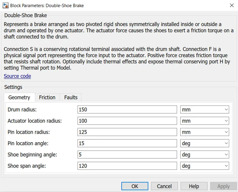
- The double-Shoe Brake block is used as a Mechanical braking system, the Sport is connected to the wheel and the force input for the Double-Shoe Brake is provided using a Gain block through an F port. The below figure shows the Block parameters of the Double-Shoe Brake
- NR and NF ports of Vehicle Body are Rear and Front normal wheel forces are connected to N signal input ports of Rear and Front tire blocks, which will apply the normal force acting on the tire.
- Connections W and beta are physical signal input ports of the Vehicle Body corresponding to headwind speed and road inclination angle respectively and are provided with the input signal using PS Constant blocks. Output signal port V gives the vehicle velocity, this output signal is logged for observation.
- Further, the Integrator block is connected to a branch from the velocity signal to get the distance travelled by the vehicle body and the output signal from the integrator is logged to observe the Distance.
Model 1-
CVT model
The below figure shows the Simscape model of BAJA ATV with Continuous Variable Transmission
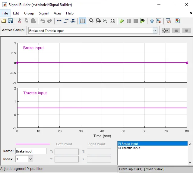
- The input signal is provided from the Signal Builder block. The Brake input is a 0 and the Throttle input is 0.5 for the entire period of 80 secs. The below figure shows the Signal Builder
- The Generic Engine takes the Speed vector and Torque vector as inputs. These input data are extracted from the Engine Torque-Speed Curve plot and defined as an array in the base workspace. The variables speed vector and torque vector are then used as input variables in the Generic Engine. The below figure shows the Engine Torque-Speed Curve plot
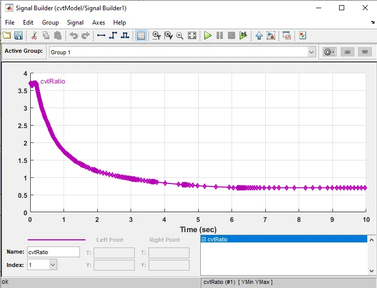
- CVT Ratio is provided to the Variable Ratio Transmission block from the Signal Builder block. The CVT Ratio is 3.7 at 0 secs and decreases to 0.7 at 10 secs. The below figure shows the CVT Ratio signal from Signal Builder
Results:
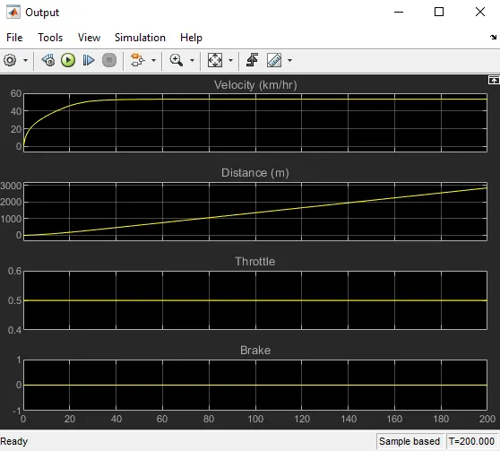
- The below figure shows the Scope Output containing Velocity, Distance, Throttle and Brake. For constant Brake and Throttle inputs of 0 and 0.5, the Velocity increases from 0 to 60 km/h in approximately 40 secs and remains 60km/h for the remaining period. For the Simulation period of 200 secs, the vehicle covers a distance of 3000 m.
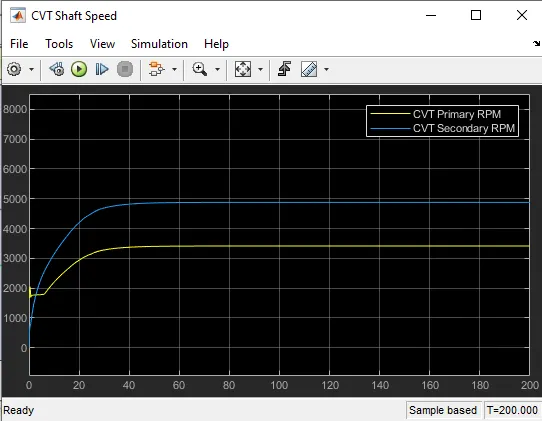
- The below figure shows the Scope output of CVT shaft speed. Initially, as the CVT ratio is high with a value of 3.7, the Primary shaft RPM is higher than the Secondary shaft RPM. After 2.8 seconds the CVT ratio falls below 1, which leads to an increase in the Secondary shaft rpm. The difference between the Primary and Secondary shaft RPM could be observed in the below figure.
Model 2-
CVT dashboard
- The below figure shows the BAJA ATV Model with Continuous Variable Transmission, which is the same as the previous model with the addition of a Dashboard
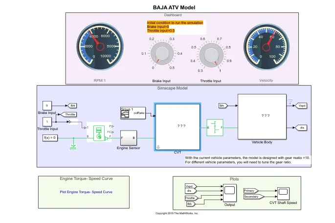
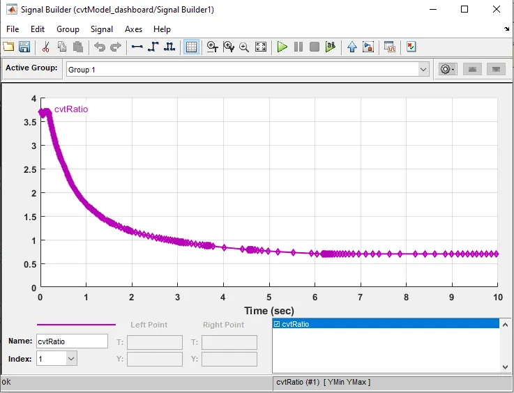
- The input is provided through Dashboard during simulation. The initial conditions to run the simulation are Brake input is 0 and Throttle input is 0.5. CVT Ratio is provided to the Variable Ratio Transmission block from the Signal Builder block. The CVT Ratio is 3.7 at 0 secs and decreases to 0.7 at 10 secs. The below figure shows the CVT Ratio signal from Signal Builder
Results-
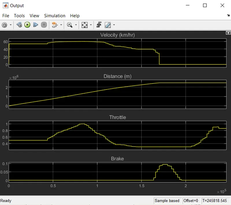
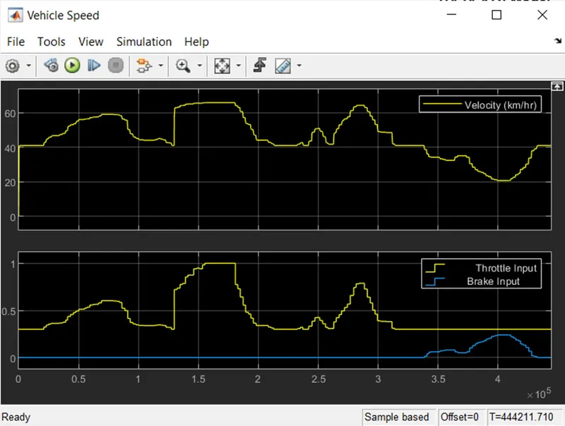
- The below figure shows the Scope Output containing Velocity, Distance, Throttle and Brake. The Throttle and Brake are varied during the simulation using the knobs inside Dashboard. The Velocity increases with an increase in Throttle and decreases with an increase in Brake and vice-versa.
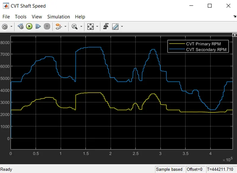
- The below figure shows the Scope output of CVT shaft speed. The Primary and Secondary Shaft RPM varies according to the Throttle and Brake inputs. RPM increases with an increase in Throttle and decreases with an increase in Brake and vice-versa.
MODEL 3-
cvtModel_cvtratio_rpm
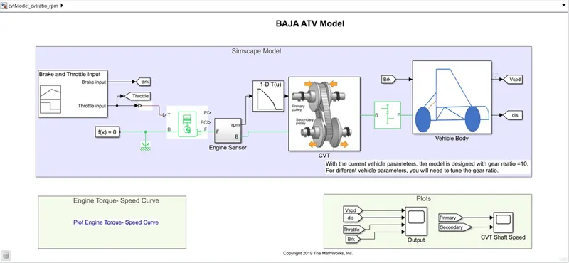
- The below figure shows the Simulink Model of BAJA ATV based on CVT ratio and engine rpm lookup table
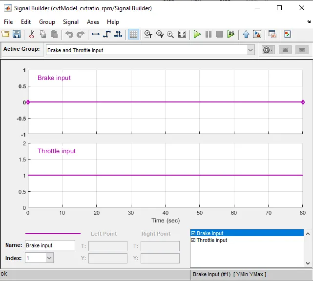
- The below figure shows the Signal Builder with Brake and Throttle input signals
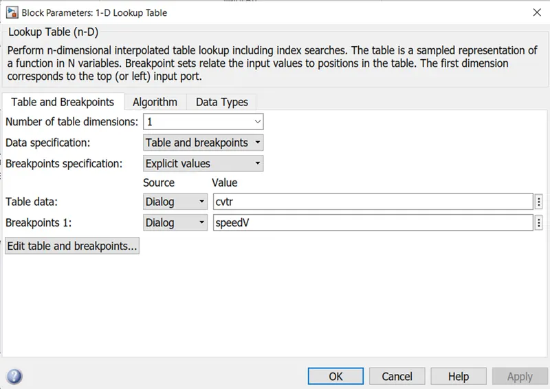
- The below figure shows the 1D Lookup table parameters. Parameters Table data and Breakpoints are provided with CVT Ratio and Engine velocity respectively. The CVT Ratio and Engine Velocity are defined in the base workspace as arrays with variable names as cover and speed respectively.
Results-
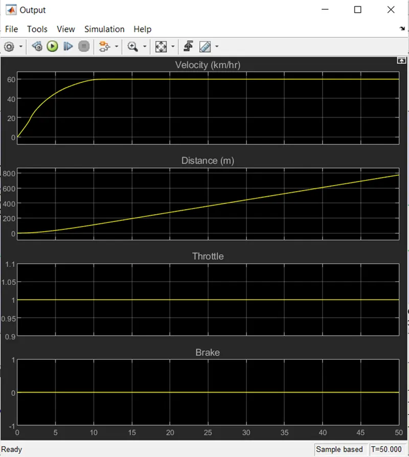
- The below figure shows the Scope Output containing Velocity, Distance, Throttle and Brake. Throttle and Brake are constant throughout the simulation with Brake input value as 0 and Throttle input value as 1. The Simulation is run for 50 secs. Velocity increases from 0 to 60 km/h in the initial 10 secs and remains the same thereafter.
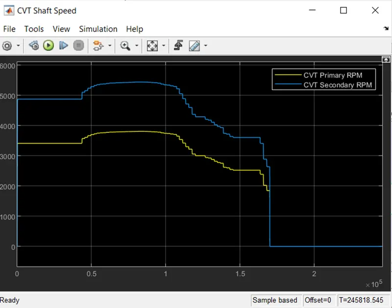
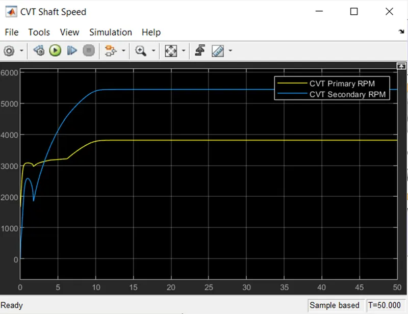
- The below figure shows the Scope output of CVT shaft speed. Initially, the Primary Shaft RPM is higher than the Secondary Shaft RPM as the CVT ratio is more than 1. After 2.8 secs the CVT ratio falls below 1 and the Secondary Shaft RPM becomes higher than the Primary Shaft RPM
MODEL 4-
cvtModel_mapped-
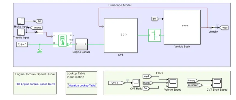
- The below figure shows the Simscape model of BAJA ATV with Continuous Variable Transmission where the CVT ratio varies based on the 1D lookup table.
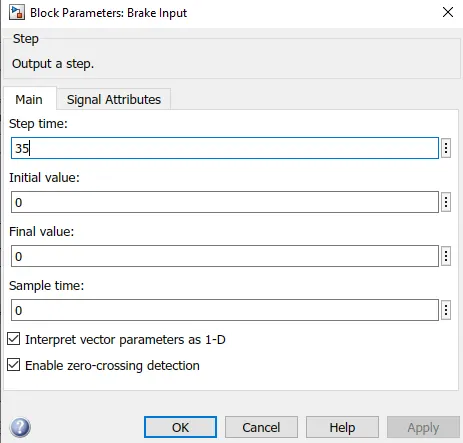
- The below figure shows Step block parameters used for Brake input. The initial and final value is 0 for a time period of 35 secs
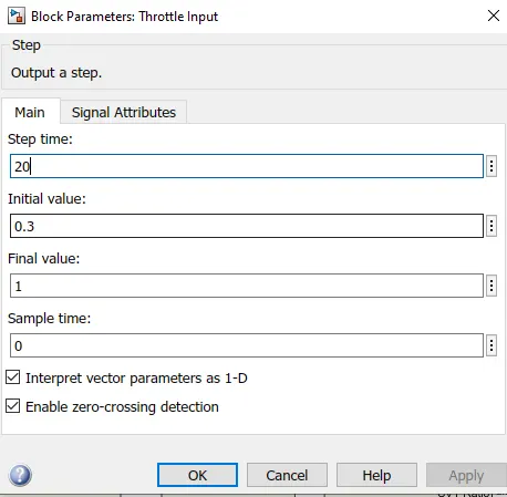
- The below figure shows the Step block parameters for Throttle input. The initial value and final value are set to 0.3 and 1 respectively with a time step of 20 secs
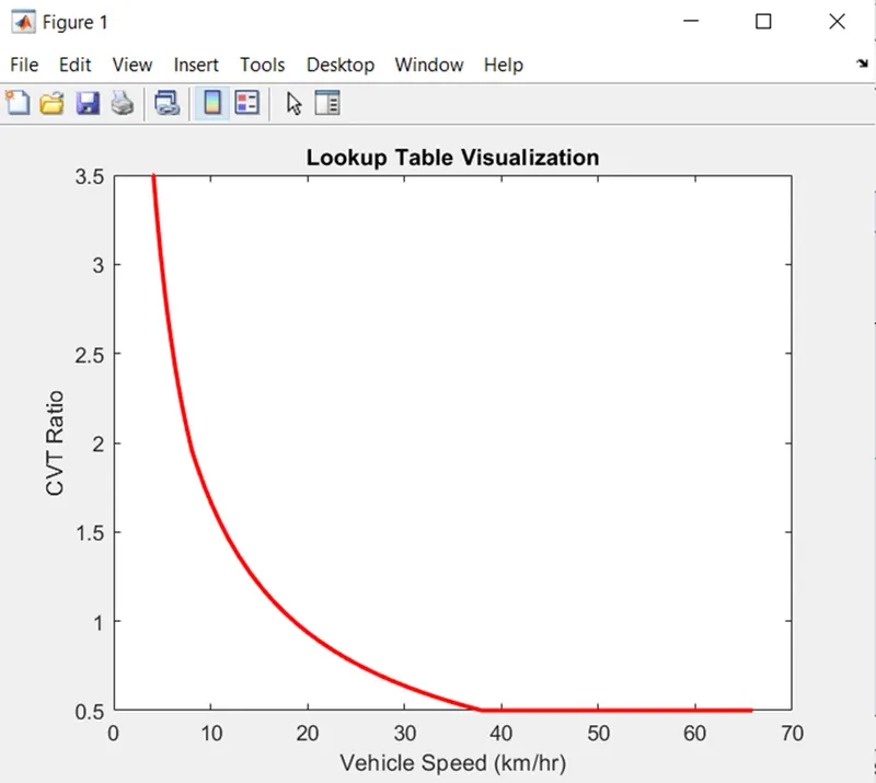
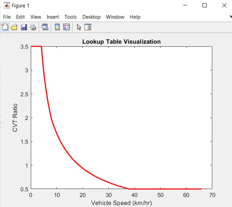
- The below figure shows the Lookup Table Visualization curve, it shows the relation between CVT Ratio and Vehicle speed
Results-
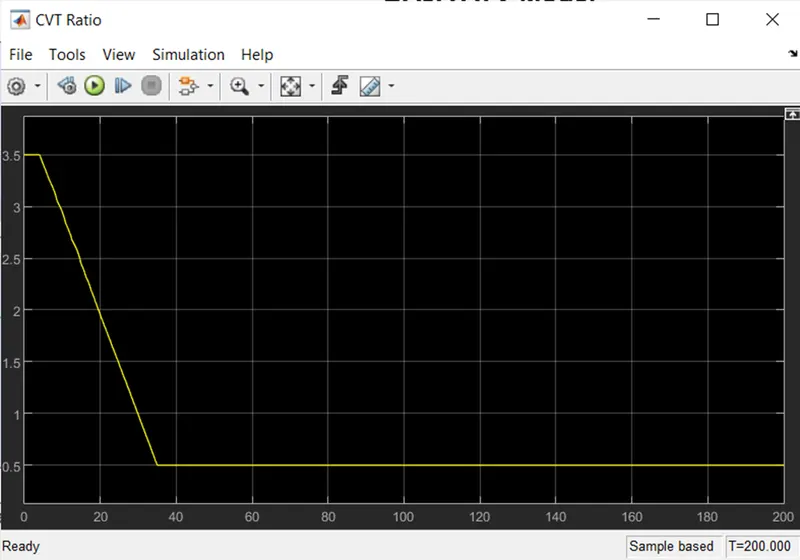
- The below figure shows the Scope output of the CVT Ratio. For the initial 4 secs the CVT Ratio is 3.5, After 4 secs the CVT Ratio decreases from 3.5 to 0.5 in the next 31 secs. After 35 secs the CVT Ratio remains constant.
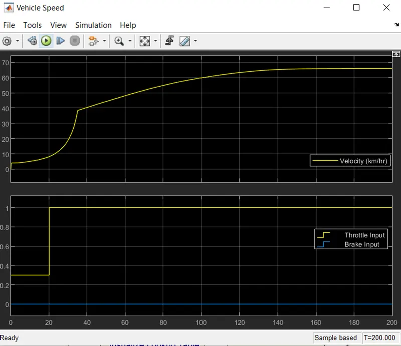
- The below figure shows the Scope output containing Vehicle Speed, Throttle input and Brake input. Brake input is 0, Throttle input is 0.3 for the first 20 secs and 1 after the first 20 secs. As CVT Ratio decreases at a high rate initially, the Vehicle speed also increases at a high rate. But after 35 secs the CVT Ratio drops to 0.5 and remains the same for the remaining time period whereas the Throttle changes from 0.3 to 1 due to which the vehicle speed increases.
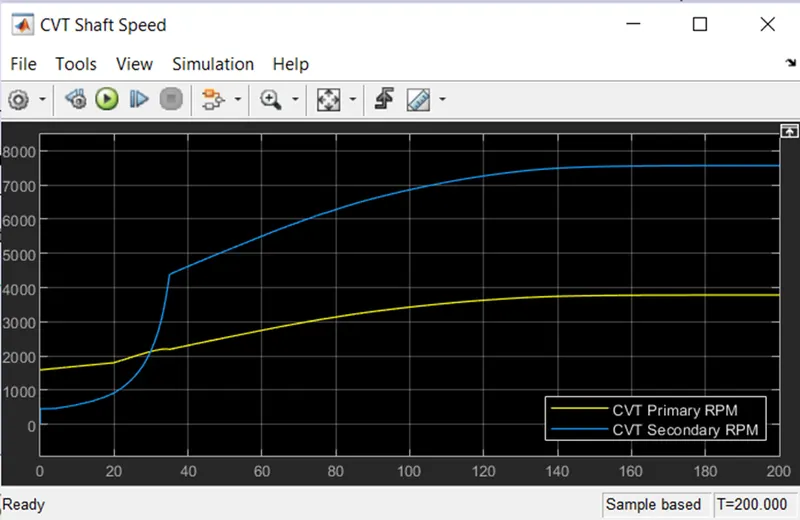
- The below figure shows the Scope output of CVT shaft speed. Initially, the Primary Shaft RPM is higher than the Secondary Shaft RPM as the CVT ratio is more than 1. After 30 secs the CVT ratio falls below 1 and the Secondary Shaft RPM becomes higher than the Primary Shaft RPM.
MODEL 5-
cvtModel_dashboard_mapped
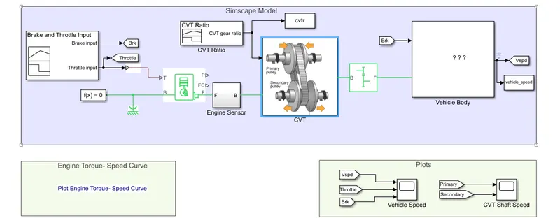
- The below figure shows the Simulink model of BAJA ATV which is the same as the previous model "cvtModel_mapped" with the addition of dashboards.
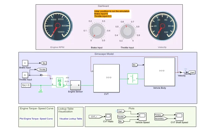
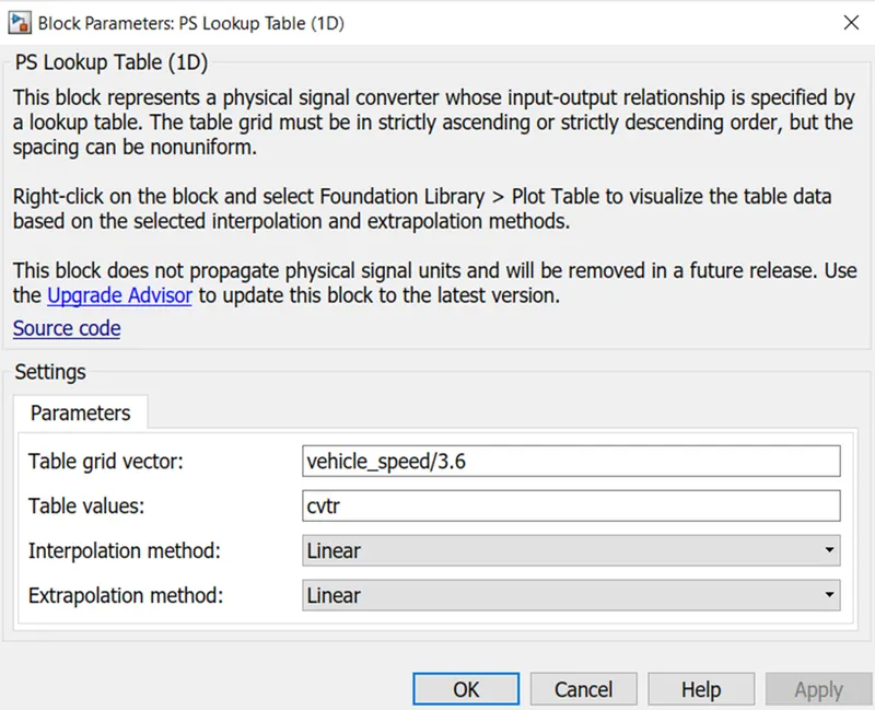
- The input is provided through Dashboard during simulation. The initial conditions to run the simulation are Brake input is 0 and Throttle input is 0.3. CVT Ratio is provided to the Variable Ratio Transmission block from the PS Lookup table. The below figure shows the PS Lookup Table block parameters
- The below figure shows the Lookup Table Visualization curve, it shows the relation between CVT Ratio and Vehicle speed
Results-
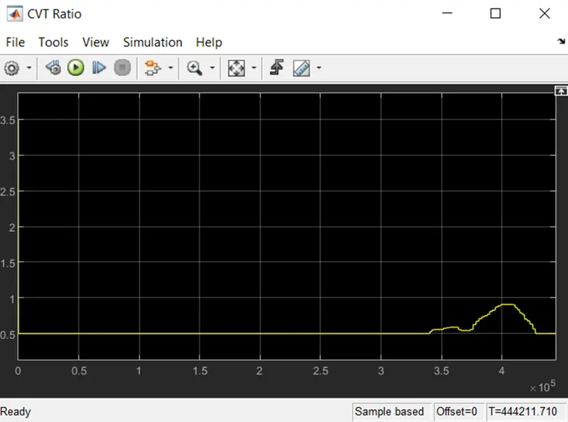
- The below figure shows the Scope output of the CVT Ratio. When the brake is applied the CVT Ratio changes accordingly.
- The below figure shows the Scope output containing Velocity, Brake input and Throttle input. Velocity increases with an increase in Throttle and decreases with an increase in Brake and vice-versa.
- The below figure shows the Scope output of CVT Shaft Speed. The CVT primary and secondary shaft ratios can be seen varying depending upon the Throttle and Brake inputs from the nature of curve comparisons.
MODEL 6-
cvtModel_data
- The below figure shows the BAJA ATV model which is used to log the CVT ratio and vehicle speed for the Lookup Table Visualization
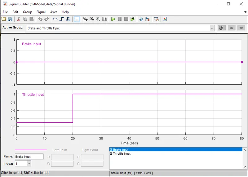
- The below figure shows the Signal Builder containing Brake and Throttle inputs. Brake input is 0, Throttle input signal is 0.3 for the first 20 secs and 1 after 20 secs for the rest of the time period.
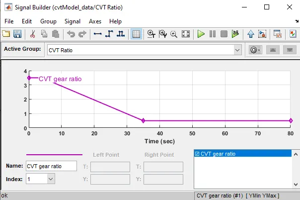
- The below figure shows the Signal Builder, using which the CVT gear ratio signal is created. CVT gear ratio is 3.5 for the first 5 secs and it decreases to 0.5 in the next 30 secs and it remains 0.5 after 35 secs.
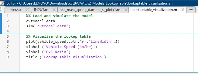
- The below figure shows the MATLAB script, which is written to load the model ‘cvtModel_data’ and run the simulation. It plots the Vehicle Speed vs CVT Ratio curve.
Results-
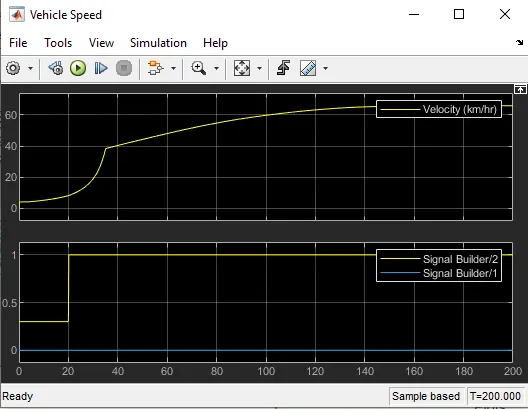
- The below figure shows the Scope output containing Velocity, Throttle input and Brake input. The Brake input is 0, Throttle input is 0.3 for 20 secs and 1 after 20 secs. Initially, Velocity increases rapidly as the CVT Ratio decreases and then the rate slows down as the CVT Ratio becomes constant and it depends only on throttle input
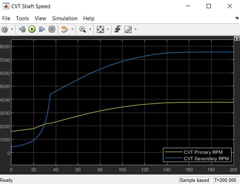
- The below figure shows the Scope output of CVT shaft speed. Initially, the Primary Shaft RPM is higher than the Secondary Shaft RPM as the CVT ratio is more than 1. After 30 secs the CVT ratio falls below 1 and the Secondary Shaft RPM becomes higher than the Primary Shaft RPM.
- The below figure shows the MATLAB script output plot of Lookup Table Visualization. The curve relates the CVT Ratio vs Vehicle Speed.
CONCLUSION-
The BAJA ATV Models with Continuous Variable Transmission have been simulated and the results were obtained and analyzed. This Models were basic and can be modified according to the requirement of realistic vehicles. There are many parameters inside the Generic Engine block which are not used in this model such as Fuel consumption and Speed control, these parameters can be used to get closer results to the real models. From the scope output plots, it can be observed that the inverse relation between the CVT Ratio and Vehicle speed. Also, when the CVT Ratio was more than 1, the Primary shaft speed was higher than the Secondary shaft speed, and when the CVT Ratio was less than 1, the Secondary shaft speed becomes higher than the Primary shaft speed.
REFERENCE-
https://drive.google.com/file/d/1b5L921zibBuSh52OdrG56DUNDaVLLWdb/view?usp=sharing