Project
Aim: Prepare a technical report explaining the model properties & comments on the results.
Theory:
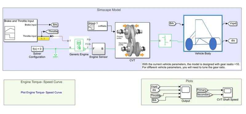
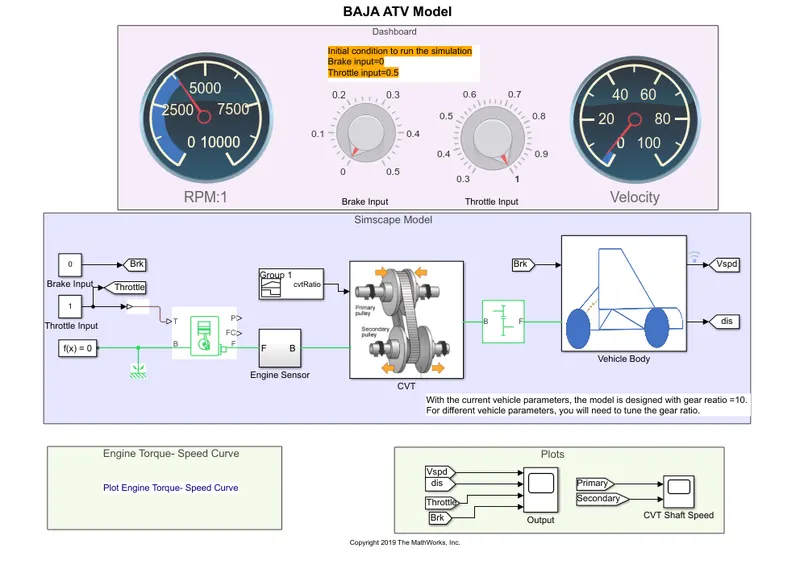
The simulation above is a working BAJA SAE model buggy which can output the velocity, displacement, throttle value, breaking input, speeds of primary and secondary CVT shaft with respect to time.
We have 2 seperate models where 1 model is a preset input model and the values can not be changed dynamically and another model can change the values dynamically inbetween the simulation to simulate real life situation where brake input and throttle input changes.
BAJA SAE:
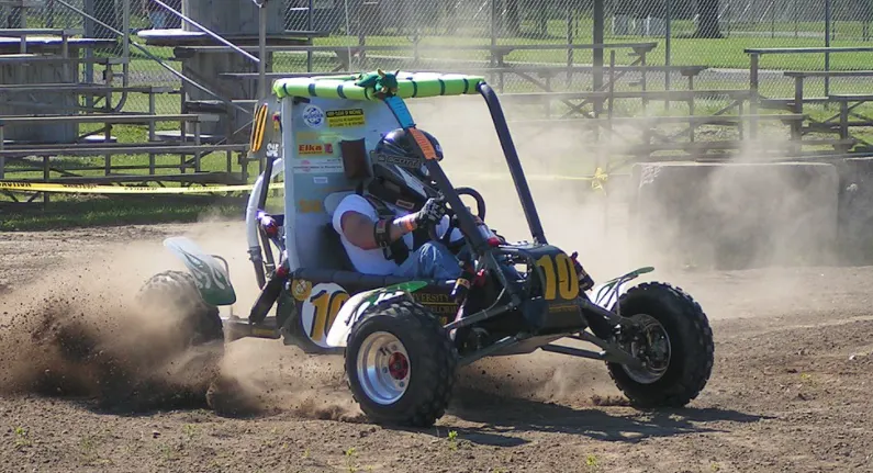
Baja SAE is an Collegiate Design Series competition run by the Society of Automotive Engineers International (SAE International). Teams of students from universities all over the world design and build small off-road cars. The cars all have engines of the same specifications. As of 2018 the engine has been an unmodified Briggs & Stratton Model 19 Vanguard engine single-cylinder with a displacement of 305cc and power output of approximately 10 bhp (7.5 kW).
The goal in Baja SAE racing is to design, build and race off-road vehicles that can withstand the harshest elements of rough terrain. The vehicles used in Baja SAE racing are often similar in appearance to dune buggies. Before 2007, the events were called "Mini Baja."
The vehicle majorly consists of a rollcage made out of circular pipes, standard engine, CVT, gearbox, break and throttle system, steering system and suspension system.
CVT:
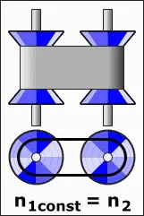
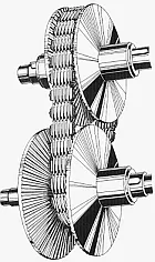
A continuously variable transmission (CVT) is an automatic transmission that can change seamlessly through a continuous range of gear ratios. This contrasts with other transmissions that provide a limited number of gear ratios in fixed steps. The flexibility of a CVT with suitable control may allow the engine to operate at a constant RPM while the vehicle moves at varying speeds.
Blocks used:
1. Signal builder: Create and generate interchangeable groups of signals whose waveforms are piecewise linear
2. From/goto blocks: Send signals to From blocks that have the specified Goto tag. If tag visibility is 'scoped', then a Goto Tag Visibility block must be used to define the visibility of the tag. The block icon displays the selected tag name (local tags are enclosed in brackets, [], and scoped tag names are enclosed in braces, {}).
3. Solver configuration: Defines solver settings to use for simulation.
4. Mechanical interference: This block represents a mechanical rotational reference point, that is, a frame or a ground. Use it to connect mechanical rotational ports that are rigidly affixed to the frame (ground).
5. Generic engine: Represents a system-level model of spark-ignition and diesel engines suitable for use at initial stages of modeling when only the basic parameters are available. Optional idle speed and red line controllers are included.
6. Subsystem: Another system with a specific output and input requirement that need not be on the main simulation block diagram
7. RPM sensor: The block represents an ideal mechanical rotational motion sensor, that is, a device that converts an across variable measured between two mechanical rotational nodes into a control signal proportional to angular velocity or angle. The sensor is ideal since it does not account for inertia, friction, delays, energy consumption, and so on.
8. Scope: Display signals generated during simulation
9. PS terminator: Use this block to terminate physical signal outputs. Unconnected physical signal output ports do not generate warnings, but connection to a PS Terminator can be used to indicate that the signal was not inadvertently left unconnected.
10. PS simulink converter: Converts the input Physical Signal to a unitless Simulink output signal.
11. Inertia input: The block represents an ideal mechanical rotational inertia.
12. Inport: Provide an input port for a subsystem or model.
13. Ideal rotational motion sensor: The block represents an ideal mechanical rotational motion sensor, that is, a device that converts an across variable measured between two mechanical rotational nodes into a control signal proportional to angular velocity or angle. The sensor is ideal since it does not account for inertia, friction, delays, energy consumption, and so on.
14. Variable ratio gear: Represents a variable ratio gearbox such as implemented by mechanical belt CVT, electric, or hydraulic transmissions. The physical signal input r defines the ratio of input to output angular shaft velocities.
15. Simple gear: Represents a fixed-ratio gear or gear box. No inertia or compliance is modeled in this block. You can optionally include gear meshing and viscous bearing losses.
16. Vehicle body: Represents a two-axle vehicle body in longitudinal motion. The block accounts for body mass, aerodynamic drag, road incline, and weight distribution between axles due to acceleration and road profile. The vehicle can have the same or a different number of wheels on each axle. Optionally include pitch and suspension dynamics or additional variable mass and inertia. The vehicle does not move vertically relative to the ground.
17. Outport: Provide an output port for a subsystem or model.
18. PS constant: This block creates a physical signal constant:
19. Integrator: Continuous-time integration of the input signal.
20. Tire (magic formula): Represents the longitudinal behavior of a highway tire characterized by the tire Magic Formula. The block is built from Tire-Road Interaction (Magic Formula) and Simscape Foundation Library Wheel and Axle blocks. Optionally, the effects of tire inertia, stiffness, and damping can be included.
21. Rotational free end: This block represents a mechanical rotational free end. Use it to allow a node to rotate freely without torque. This block can be used to optionally specify initial rotational velocity.
22. Gain: Element-wise gain (y = K.*u) or matrix gain (y = K*u or y = u*K).
23. Double shoe brake: Represents a brake arranged as two pivoted rigid shoes symmetrically installed inside or outside a drum and operated by one actuator. The actuator force causes the shoes to exert a friction torque on a shaft connected to the drum.
24. Knob: Set a value to tune parameters or variables.
25. Custom gauge: Display an input value on a customized gauge.
Procedure:
CVTmodel:
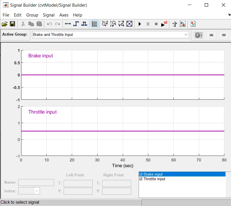
1. The brake and throttle input are simulated with signal builder and a value vs time input is simulated for 80 sec.
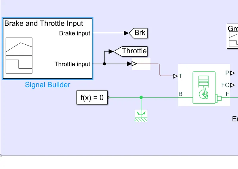
2. The break and throttle output are connected with goto blocks that will directly feed into the vehicle body and scopes in later stages.
3. The throttle output is then also connected to a PS simulink converter and fed to a generic engine block.
4. The engine block is connected with a solver configuration, mechanical refrence and gives a mechanical output, The throttle input signal T lies between zero and one and specifies the torque demanded from the engine as a fraction of the maximum possible torque. Connections F and B are mechanical rotational conserving ports associated with the engine crankshaft and engine block, respectively. Connections P and FC are physical signal output ports through which engine power and fuel consumption rate are reported. the output F i.e., mechanical observer port is sent to a subsystem that will act as an engine sensor.
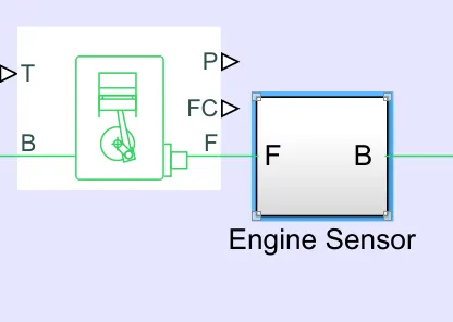
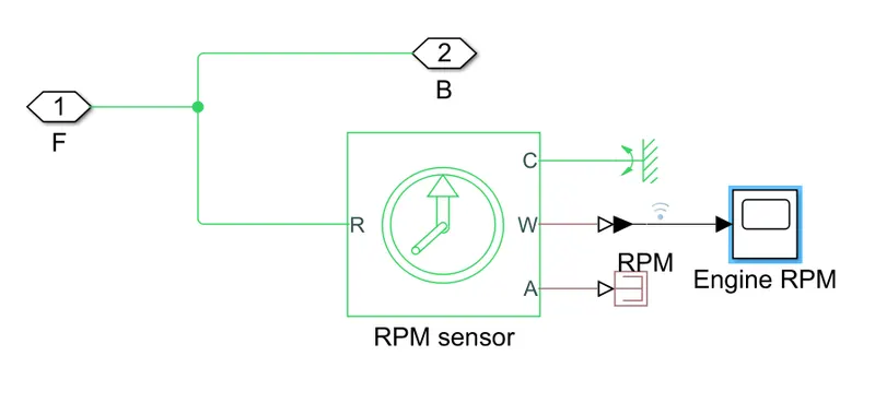
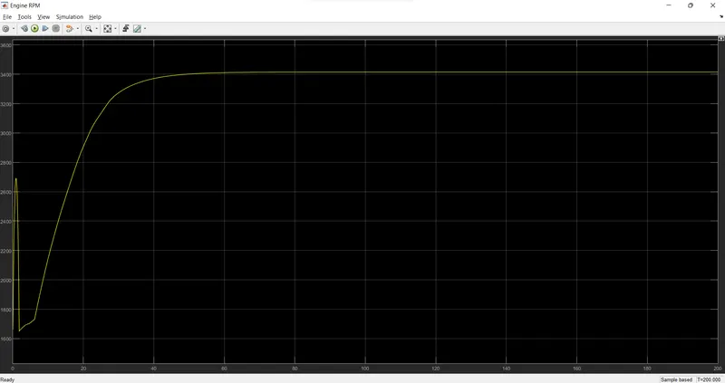
5. The input and output are the same i.e., the crankshaft output and is directly sent as an output to the CVT, the input however is used to figure out the engine RPM w.r.t. time, it is connected with a mechanical reference and at the output mechanical conserving port, whilst the scope is connected to the velocity output with the help of PS simulink converter that is the RPM w.r.t. time and the PS terminator to the angular displacement to terminate the angular displacement signal.
6. The CVT subsystem has two inputs,
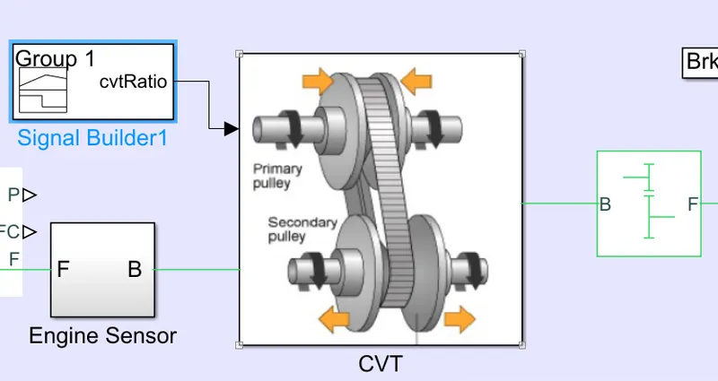
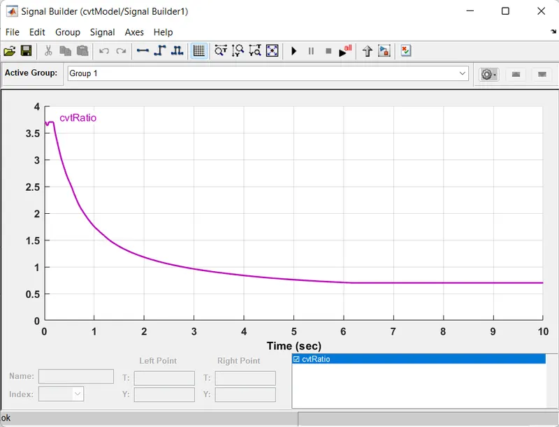
a. the CVT ratio via the signal builder simulating the ratio vs time for a range of 10 sec,
b. the second input is the engine input that is coming from the generic engine,
Then the inputs are fed to a variable ratio gear where the gear acts as a CVT and the CVT ratio is connected via an inport to the r input port where r defines the ratio of input to output angular shaft velocities.
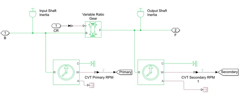
B and F are mechanical conserving ports acting as input and output respectively.
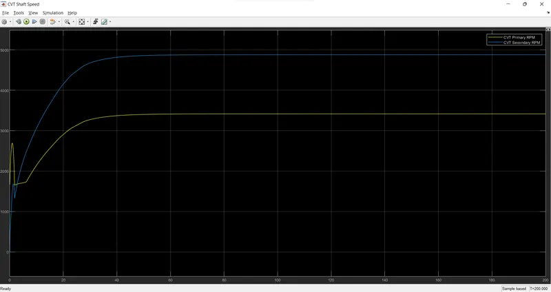
The B signal is connected with an input shaft inertia block anf an RPM sensor before connecting to the gear. where the input shaft inertia acts as the primary CVT and the sensor is for the sake of monitoring the RPM of the same and is connected with a mechanical reference, goto block that feeds into a from block into a scope on the main diagram, and a PS terminator.
The output F is connected to a similar arrangement, where the RPM is monitored with a sensor that feeds to a scope on the main diagram and the output F is connected to output shaft inertia block of secondary CVT that furrther gives the main output afterwards.
7. The output is then fed to a simple gear which has a gear ratio of for the sole purpose of increasing the torque to the vehicle body.
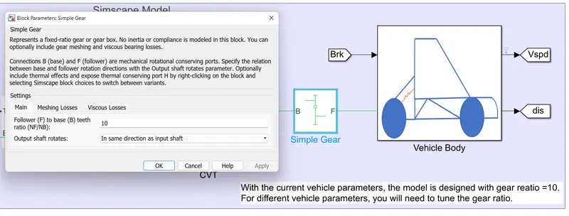
8. The next block is the subsystem vehicle body that has the input from the simple gear and the brake from the input from the first signal builder,
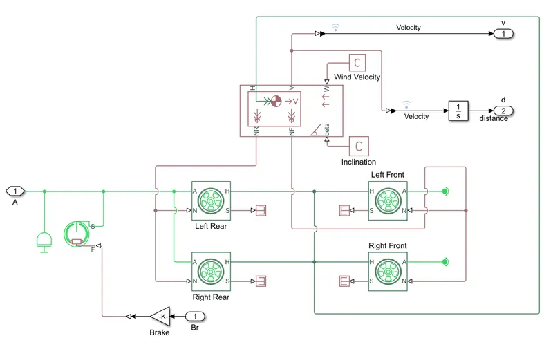
The vehicle body consists of 4 tires(magic formula), vehicle body block and a double shoe brake block.
The break input feeds to a gain block with 1000 gain value that is further converted with the help of PS simulink converter block and fed to the input of the double shoe brake block.
The input is connected with the brake block output and is now sent to the Rear tires simultaneously to port A, Connection A is the mechanical rotational conserving port for the wheel axle. Connection H is the mechanical translational conserving port for the wheel hub through which the thrust developed by the tire is applied to the vehicle. Connection N is a physical signal input port that applies the normal force acting on the tire. The force is considered positive if it acts downwards. Connection S is a physical signal output port that reports the tire slip.
The front tires are given input from the H ports of the rear tires to the H port of front tires to simulate transversal motion from the thrust of rear tires. The A ports a connected to a rotation free end to simulate free end and a dead axle.
9. The vehicle body block recieves the resulting traction motion developed by tires in port H. Connections V, NF, and NR are physical signal output ports for vehicle velocity and front and rear normal wheel forces, respectively, where V is fed to the outport to act as an output i.e., vehicle velocity and further more, the same output is connected to an integrator which converts the velocity into the distance travelled and feeds into another outport that'll be distance output.
The wheel forces are fed in to the respective tires.
Connections W and beta are physical signal input ports corresponding to headwind speed and road inclination angle, respectively and are fed from PS constant blocks that give the value 0.
The whole contraption gives the value of vehicle velocity and distance travelled as output.
10. The output from the vehicle body are fed to goto blocks which feed into the same scope connected to the throttle and break input.
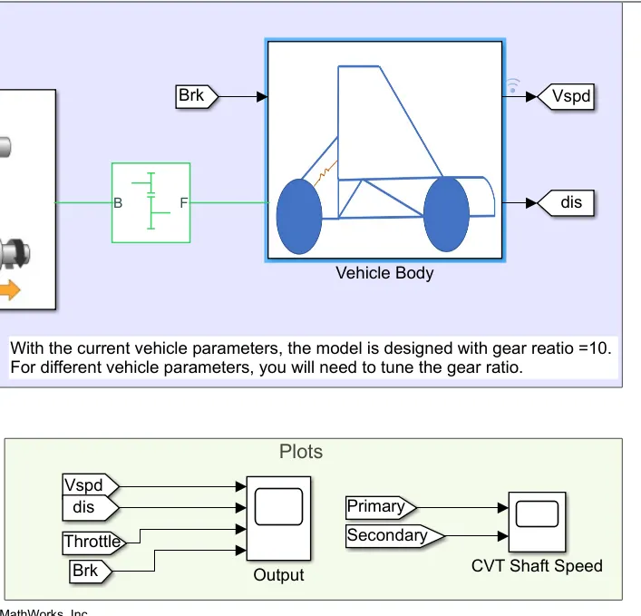
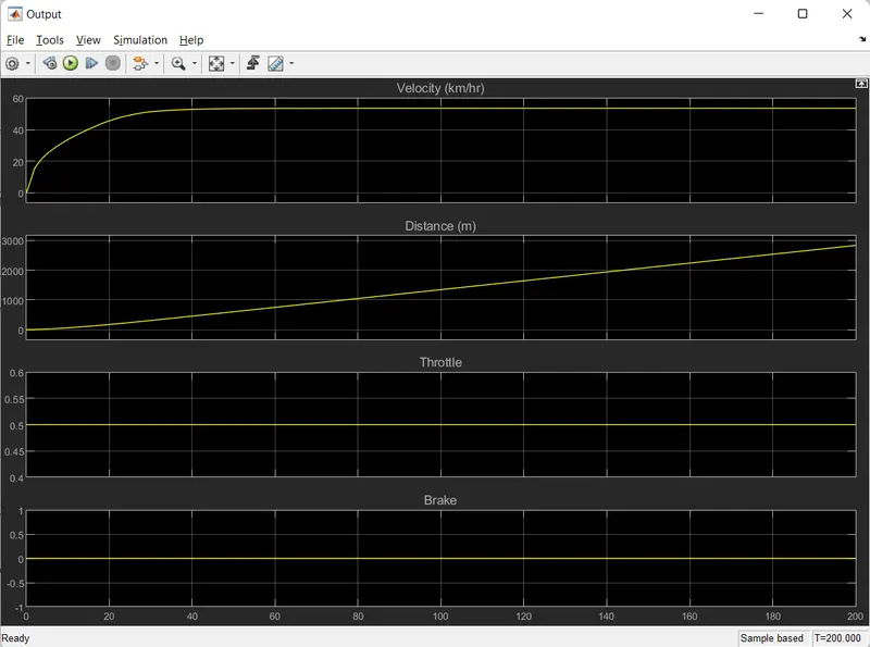
11. The whole model is arranged such that the plots of vehicle speed, throttle input, distance travelled and break input are next to the plot of secondary and primary CVT RPM.
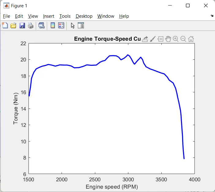
12. The plot of engine torque vs RPM is plotted as well.
13. The simulation is ran for 200 sec.
Results:
The plot of engine torque vs RPM is achieved,
The plots of vehicle speed, throttle input, distance travelled and break input w.r.t. time are achieved
The plots of econdary and primary CVT RPM w.r.t. time are achieved
The plot of engine RPM w.r.t. time is achieved
CVTmodel with dashboard:
Procedure:
1. Everything is the same as the previous model but the inputs have been changed from constant preset inputs to knobs that can control the throttle and brake input,
2. The knobs are controlling the constant block which feed the values to the respective throttle and brake input blocks
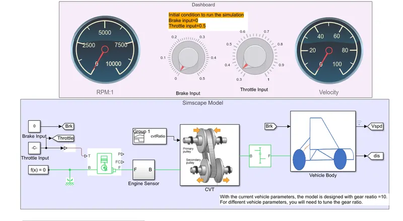
3. We can adjust the knobs and create a dynamic simulation to acheive real like results.
Results:
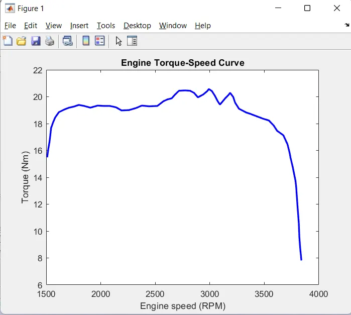
The plot of engine torque vs RPM is achieved, it remains the same as it is the property of the engine and is not influenced by the external factors such as speed and brake input
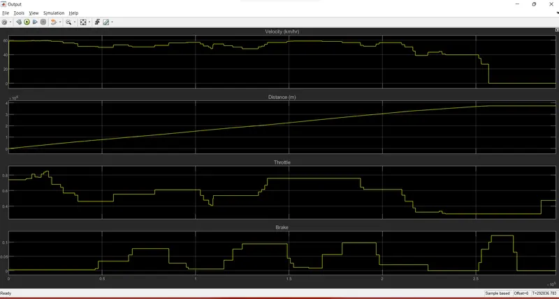
The plots of vehicle speed, throttle input, distance travelled and break input w.r.t. time are achieved
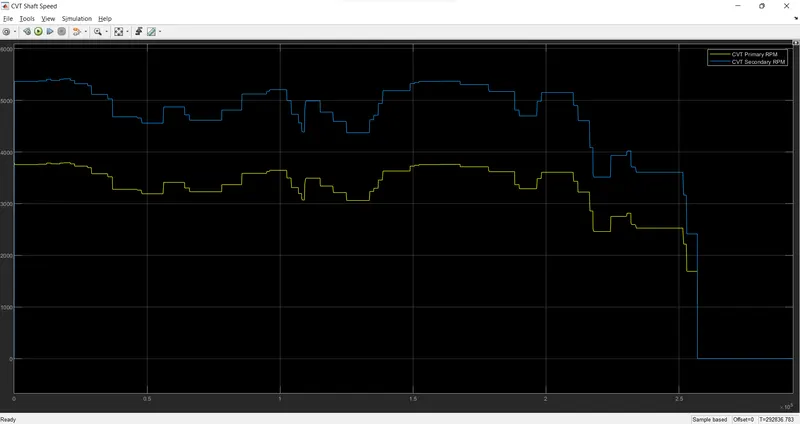
The plots of secondary and primary CVT RPM w.r.t. time are achieved
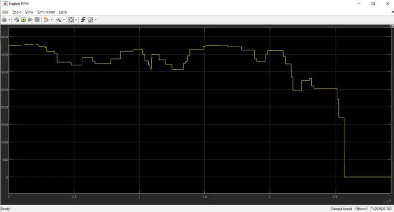
The plot of engine RPM w.r.t. time is achieved
Conclusion:
We can simulate a BAJA SAE vehicle and successfully implement the results for improvement in the design if necessary.
Drive link: