Week 4.1 - Genetic Algorithm
Aim: To write a code in MATLAB to optimise the stalagmite function and find the global maxima of the function, explain genetic algorithm and it's syntax, and plot Fmax vs no. of iterations graph.
A genetic algorithm (GA) is a method for solving both constrained and unconstrained optimization problems based on a natural selection process that mimics biological evolution. The algorithm repeatedly modifies a population of individual solutions. At each step, the genetic algorithm randomly selects individuals from the current population and uses them as parents to produce the children for the next generation. Over successive generations, the population "evolves" toward an optimal solution and generates the global minima of the used function.
You can apply the genetic algorithm to solve problems that are not well suited for standard optimization algorithms, including problems in which the objective function is discontinuous, nondifferentiable, stochastic, or highly nonlinear.
The following outline summarizes how the genetic algorithm works:
-
The algorithm begins by creating a random initial population.
-
The algorithm then creates a sequence of new populations. At each step, the algorithm uses the individuals in the current generation to create the next population. To create the new population, the algorithm performs the following steps:
-
Scores each member of the current population by computing its fitness value. These values are called the raw fitness scores.
-
Scales the raw fitness scores to convert them into a more usable range of values. These scaled values are called expectation values.
-
Selects members, called parents, based on their expectation.
-
Some of the individuals in the current population that have lower fitness are chosen as elite. These elite individuals are passed to the next population.
-
Produces children from the parents. Children are produced either by making random changes to a single parent—mutation—or by combining the vector entries of a pair of parents—crossover.
-
Replaces the current population with the children to form the next generation.
-
-
The algorithm stops when one of the stopping criteria is met such as Maximum number of generation, time, fitness limit and some more have been reached.
-
The algorithm takes modified steps for linear and integer constraints(including bounds), the algorithm modifies the evolution of the population to be feasible with respect to to the constraints and there are special functions that need to be created in case there is only one constraint values such as mutation and crossover manually to make the solution feasible.
-
The algorithm is further modified for nonlinear constraints such that the GA uses augmented langrangian genetic algorithm to solve non linear constraint problems without intergal constraints and another one that we used that is penalty algorithm where to evaluate the fitness, ga computes a penalty as a value for some conditions and attempts to create a feasible population of the GA.
Syntax of GA:
x = ga(fun,nvars)x, to the objective function, fun. nvars is the dimension (number of design variables) of fun.
x = ga(fun,nvars,A,b)x to fun, subject to the linear inequalities A*x ≤ b. ga evaluates the matrix product A*x as if x is transposed (A*x').
x = ga(fun,nvars,A,b,Aeq,beq,lb,ub,nonlcon)nonlcon. The function nonlcon accepts x and returns vectors C and Ceq, representing the nonlinear inequalities and equalities respectively. ga minimizes the fun such that C(x) ≤ 0 and Ceq(x) = 0. (Set lb=[] and ub=[] if no bounds exist.)
Writing the given equation as a stalagmite function:
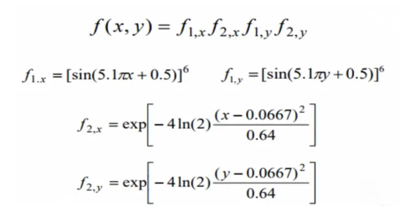
The function code is used in the main functions below as an equation code and the function has been given a negative sign to reverse the effects of the GA function to produce maxima value instead of minima value as desired.
function[f] = stalagmite(input_value)

x = input_value(1);
y = input_value(2);

f1_x = (sin(5.1*pi*x + 0.5)).^6;
f1_y = (sin(5.1*pi*y + 0.5)).^6;
f2_x = exp(-4*log(2)*((x-0.0667).^2/(0.64)));
f2_y = exp(-4*log(2)*((y-0.0667).^2/(0.64)));

f = -(f1_x.*f2_x.*f1_y.*f2_y);
end
Writing the Main functions for GA for unbounded statistical behavior:
1. Start by inputting the vector array for the x and y axes,
2. Define a number for the iterations to be ran,
3. Create a mesh using meshgrid from the input vectors to define a search space for the maxima of the function,
4. Write a for loop for the length of x vector array and then write a for loop for the length of y vector array for each iteration of length of x vector in the loop itself to run the function through each input value of the mesh array and define the function(stalagmite) for the i and j input vlaues thus calculating the fitness of each and every value of the meshgrid,
5. Then plot a surface using surface command followed by a negative sign on the function input to invert the direction of the plot because the function is defined in negative direction giving positive value to the maxima function.
6. Now write the code for unbounded statistical behavior,
7. Using the syntax of ga(@stalagmite,2) | ga(fun,nvars) for an unconstrained values and unbounded behavior with the help of for loop to find the optimum value for each iteration.
8. Using the tic toc command to measure the time taken to complete the study,
9. Using the figure command to open the figure window and subplot command to get multiple plot in the same window where the fopt plot is plotted to generate the Fmax value vs no. of iterations graph, now use plot3 command to obtain the 3D surface and use label and marker commands as needed.
10. The same process from 7-9 wil ve followed for the bounded and penalty algorithm approach where the ga syntax is changed as x=ga(@stalagmite,2,[],[],[],[],[0;0],[1;1]) | x = ga(fun,nvars,A,b,Aeq,beq,lb,ub)x = ga(fun,nvars,A,b,Aeq,beq,lb,ub,nonlcon,options)
11. The third case has additional command options=optimoptions('ga','populationsize',300) to increase the size of the population and generate a fesible result.
clear myfunc
close all
clc

%Inputs and the population space
x = linspace(0,0.6,150);
y = linspace(0,0.6,150);
%Number of cases to be ran
num_spaces = 50;

%creating an array from the x and y array values

[X, Y] = meshgrid(x,y);

%Writing a loop to run all values of x and y for the function
for i = 1:length(X)
    for j = 1:length(Y)
        input_value(1) = X(i,j);
        input_value(2) = Y(i,j);
        %Values of each function in the defined space
        f(i,j) = stalagmite(input_value);
    end
end

%plotting the function as surface
surfc(X,Y,-f);
shading interp


%%Unbounded statistical behavior
%calculating the study time through tic and toc command
tic
for i=1:num_spaces
%Calculating the function's optimum value
[inputs,fopt(i)] = ga(@stalagmite,2)
%At every iteration
xopt(i)=inputs(1);
yopt(i)=inputs(2);
end

%Displaying time taken
study1_time = toc

%Plotting
figure
subplot(2,1,1)
surfc(X,Y,-f);
hold on
shading interp
plot3(xopt,yopt,-fopt,'marker','square','markersize',8,'markerfacecolor','r');
xlabel('x');
ylabel('y');
grid on
subplot(2,1,2)
plot(-fopt);
xlabel('iterations')
ylabel('function max value')


%%Bounded statistical behavior
%calculating the study time through tic and toc command
tic
for j=1:num_spaces
%Calculating the function's optimum value
[inputs,fopt(j)]=ga(@stalagmite,2,[],[],[],[],[0;0],[1;1])
%At every iteration
xopt(j)=inputs(1);
yopt(j)=inputs(2);
end

%Displaying time taken
study2_time=toc

%Plotting
figure
subplot(2,1,1)
surfc(X,Y,-f)
hold on
shading interp
plot3(xopt,yopt,-fopt,'marker','square','markersize',8,'markerfacecolor','r');
xlabel('x');
ylabel('y');
grid on
subplot(2,1,2)
plot(-fopt);
xlabel('iterations')
ylabel('function max value')


%%Modifying the number of population
%Increaing the sixe of population by using optimoptions function
options=optimoptions('ga','populationsize',300)
%Calculating the study time through tic and toc command
tic
for k=1:num_spaces
%Calculating the function's optimum value
[inputs,fopt(k)]=ga(@stalagmite,2,[],[],[],[],[0;0],[1;1],[],[],options)
%At every iteration
xopt(k)=inputs(1);
yopt(k)=inputs(2);
end

%Displaying time taken
study3_time=toc

%Plotting
figure
subplot(2,1,1)
surfc(X,Y,-f)
hold on
shading interp
plot3(xopt,yopt,-fopt,'marker','square','markersize',8,'markerfacecolor','r');
xlabel('x');
ylabel('y');
grid on
subplot(2,1,2)
plot(-fopt);
xlabel('iterations')
ylabel('function max value')
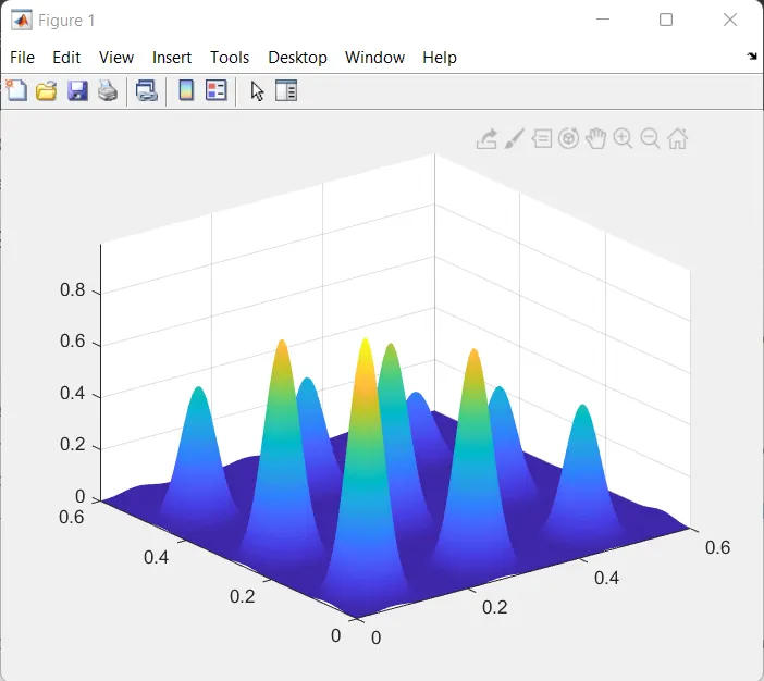
Results: The results obtained for the initial function are
The graph for the unbounded behavior study are below
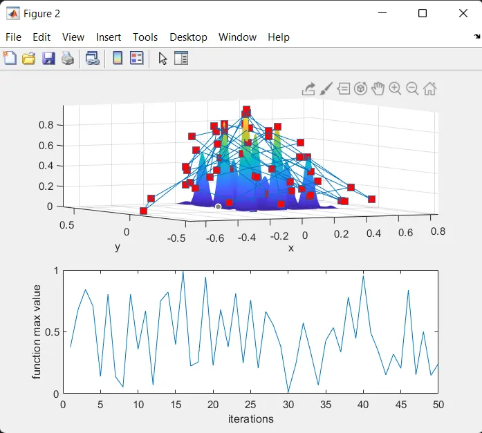
Time to study: 2.33 seconds
The graph for bounded behvior study are
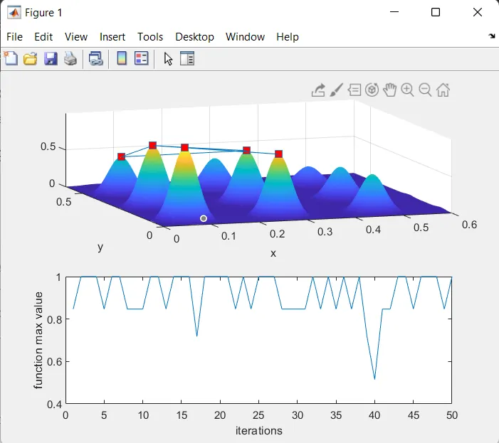
Time to study: 3.04 seconds
The graph for penalty algorithm study are
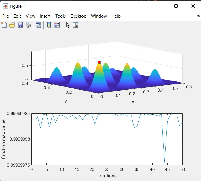
Time to study: 14.01 seconds
Conclusion: The increase in population size increased the precision of value of global maxima.
The global maxima = 1
Note: No important errors were encountered
Reference: Mathworks help center.