Week 3 - Solving second order ODEs

Explaining the code:

1. We start the code by specifying the given inputs

2. the next step is to define the staring condition of the pendulum namely displacement and velocity in terms of angles in radians.

3. We generate an array for the time span of the simulation with the given time frame.

4. We solve the second order ODE in terms of time and results by using ode45 function of MATLAB and using our defined ode_function in terms of defined and calculated terms

5. Ode45 is the function of time(t) and angles(theta) i.e., dependent and independent variables followed by our simplified function of the second order ODE into 2 single order ODE by ode_function in conjunction with given constants or inputs parameters followed by initial conditions and integrations namely time array and angles.

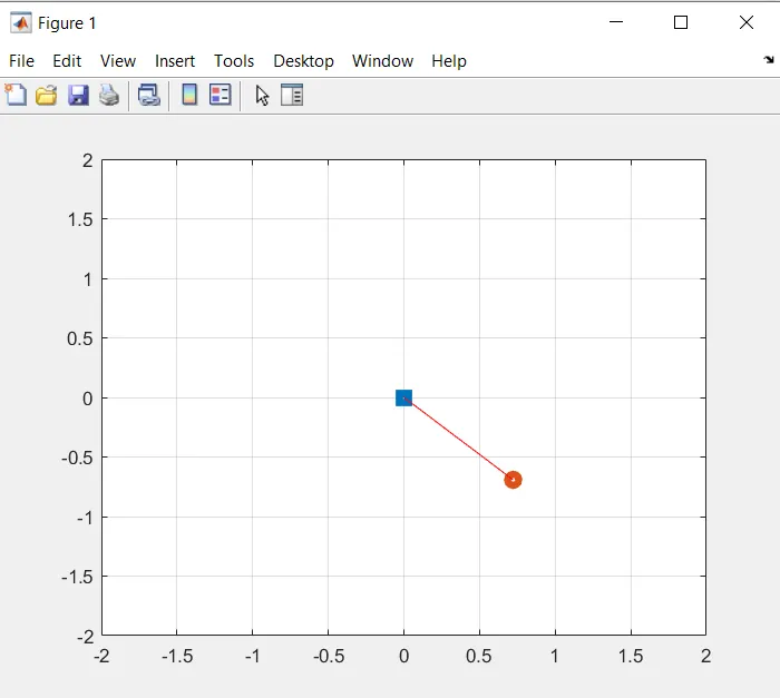
6. the next step is to write a for loop program with predefined positions of the hinge to generate multiple values of the postion of the pendulum in conjunction to the results to generate an animation of the same to simulate the whole mechanism of the pendulum in discussion.

7. The generated animation is converted into an avi file with getframe and writevideo command.

clear all
close all 
clc 

%Solving second order ODE for a simple pendulum 

%Inputs
L = 1;
m = 1;
b = 0.05;
g = 9.81;

%defining the initial condition of the pendulum as given 
theta_0 = [0;3];

%Defining the time span array of the simulation 
t_array = linspace(0,20,1000);

%Solving the ODE for a defined function 
[t, results] = ode45(@(t, theta) ode_function(t,theta,L,m,b,g),t_array,theta_0);


%Looping for Generating animation of moving pendulum 

        x0 = 0;
        y0 = 0;

        videoFile = VideoWriter('pendulum.avi','Uncompressed AVI');
        open(videoFile);

for i = 1:length(results(:,1))

        
        y1 = -L*cos(results(i,1));
        x1 = L*sin(results(i,1));

        %Plotting
        figure(1)
        plot(x0,y0,'marker','square','LineWidth',4)
        hold on
        plot(x1,y1,'marker','o','LineWidth',4)
        plot([x0 x1],[y0 y1],'r')
        axis([-2 2 -2 2])
        grid on
        pause(0.03)
        writeVideo(videoFile,getframe(gcf));
        clf;
       

end
close(videoFile)

Explaining the function:

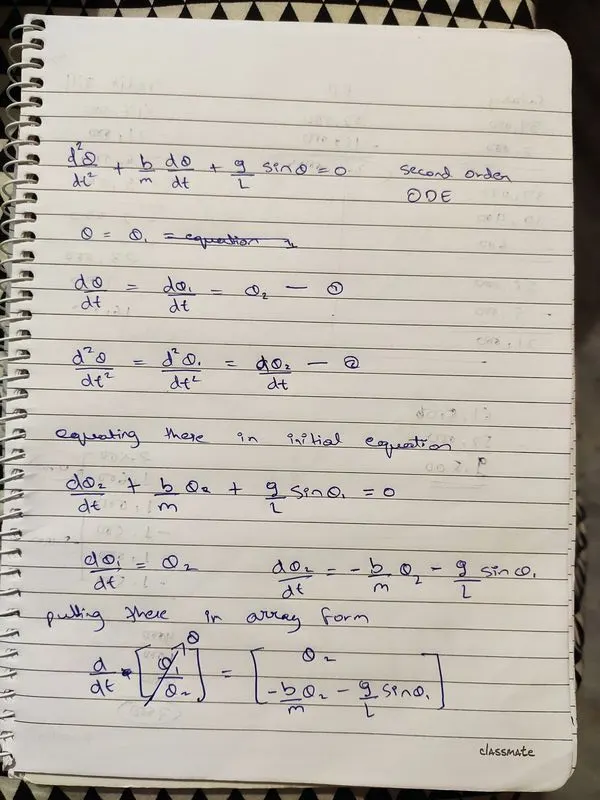
1. The second order ODE can be solved by converting it into two single order ODE and that can be done by introducing a new angular variable so that it can substitute the second order values to be single order

2. The new variable is defined in the code and two equations are generated.

3. The two generated equations are equated in terms of dtheta2_dt in an array to determine dtheta_dt .

4. This function is written to take inputs from the given values.

logic behind the solution - 

function code-

function [dtheta_dt] = ode_function(t,theta,L,m,b,g)

theta1 = theta(1);
theta2 = theta(2);
dtheta1_dt = theta2;
dtheta2_dt = -(b/m)*theta2 - (g/L)*sin(theta1);
dtheta_dt = [dtheta1_dt; dtheta2_dt];
end

Generated figure:

Results:

An animation is generated of the whole simulation and the drive link is attached below

https://drive.google.com/drive/folders/13tAoOcUTH7dZtErhleRAdix6TUqabWwo?usp=sharing

errors faced: 

The avi file was corrupted

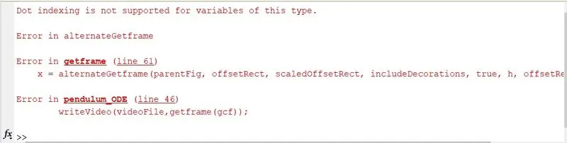
Solution and assesment - The error was faced because the function was taking too long to generate the avi file and was being terminated, it was solved by shortening the time of the simulation.