Simulation of an All Terrain Vehicle (ATV) with a Continuous Variable Transmission - Final Project
BAJA ATV Model: The model of an All-terrain Vehicle (ATV) with a Continuous Variable Transmission (CVT) is developed, and the effect of different throttle and brake inputs on the vehicle performance and CVT pulleys speed is observed. The major aim is to compare the two sets of model - an open loop model wherein the CVT ratio is given through a signal builder block and hence is pre-determined as a function of time. The other model is a closed-loop model, wherein the CVT ratio is given through a lookup table, where the CVT ratio is a function of the vehicle speed. The other variation is the presence and the absence of the Dashboard. The presence of the dashboard allows to manually vary the input throttle and brake inputs in real-time during the simulation. Hence, all the four variations of the model is simulated and the results are intepreted.
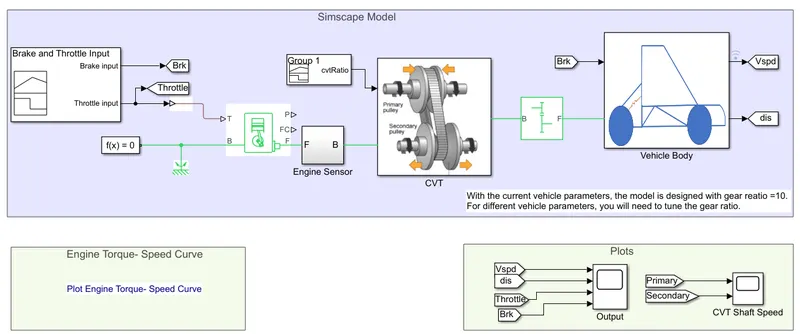
Model 1 : The model is an open-loop model, wherein the CVT Ratio for the entire simulation is given as an direct input, and not a feedback signal. Hence, the model is open-loop model.
Reference : https://in.mathworks.com/matlabcentral/fileexchange/70576-baja-all-terrain-vehicle-atv-model.
The major components in the model includes :
Generic Engine : The simscape block represents a general internal combustion engine (Spark ignition and Diesel). Basically, an Engine is an energy converter which converts the chemical energy of the fuel into pressure energy which in-turn is converted into mechanical energy. The IC engine is a type of engine wherein the ignition and combustion of the fuel takes places within the combustion chamber. It is the system-level model of an engine based on basic parameters used at the early stages of modeling the system. The parameterization of the model can be provided either through speed-power or speed-torque data. In this case, the input speed and torque vectors are given. If more detailed model is to be created, the fuel consumption maps and the idle speed controllers can be includes. However, in this model those data is not included.
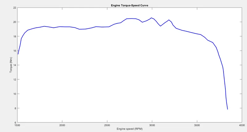
The T signal is the throttle input signal which specifies the torque demand as a fraction of the maximum torque. Connections B and F are the mechanical rotational conserving ports, hence the B is connected to a mechanical rotational reference and F is the follower, connected to the next block. The primary input data for the model, includes the speed and torque vectors. The engine speed-torque plot is as shown below. The grabit function is used in the model to determine the data-points from the image, and is fed as input into the generic engine block. The other data includes the engine inertia (0.008 kgm^2) and initial velocity.
Engine sensor : The block setup is as follows, which measures the RPM of the engine crankshaft at every time-step. Hence, this block outputs the Engine RPM.
Continuous Variable Transmission (CVT): A CVT is an transmission that can select any desired drive ratio within its operating range. The major components of the CVT includes the primary pulley (input) , secondary pulley(output) and a metal belt. Both these pulleys are of variable-diameter type. The driving pulley is connected to the engine crankshaft, while the driven pulley transfers the motion to the drive shaft.
These pulleys have two cones, and the belt is placed in the groove in between the two cones. When the two cones come close towards each other, the belt rides higher on the grooves, and hence the pulley diameter is increased, whereas when the pulley cones pulls away, then the belt rides lower and hence the diameter reduces. On the other hand, when the diameter of the driven pulley increases, then the diameter of the driving pulley decreases and vice-versa. As the pulleys change diameters relative to each other, an infinite series of gear ratios is obtained.
For example : When the diameter of the driving pulley is small, and the diameter of the driven pulley is large, then it is said to be in a lower gear, produces more torque. Where in a vice-versa condition, where the diameter of the driven pulley is large and the diameter of the driving pulley is small, then it is said to be in a higher gear. The CVT model is as follows :
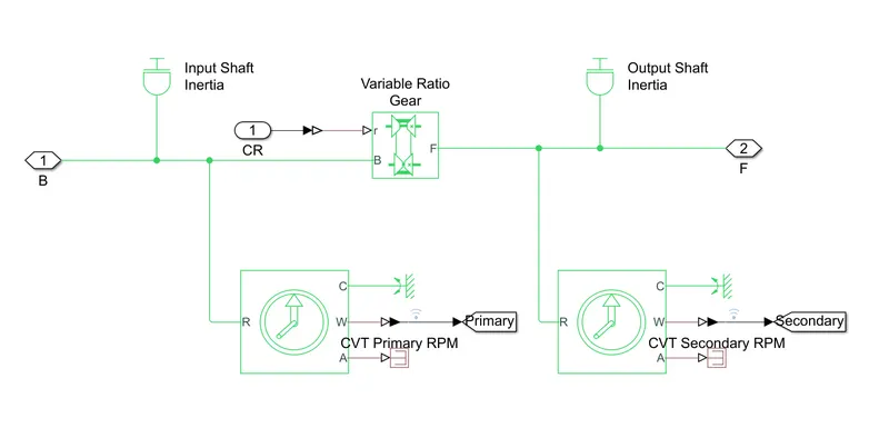
In the above model, the CVT is represented by the variable ratio transmission block. The B is the base and hence is connected to the engine crankshaft. Whereas the driven pulley is the follower, and hence the F connection port denoting the follower is the output. The transmission stiffness and damping of the base connection is set as per the vehicle specifications. The transmission and viscous losses are neglected in this model. The inertia blocks are connected to represent the input and output shaft inertias ( shafts of the driving and driven pulleys respectively), and even the rotational sensors are used to measure the primary(input/driving) pulley and secondary (output/driven) pulley RPM. The driven pulley is connected to the simple gear block with a constant gear ratio, which can be used to represent the differential reduction or a combination of a gear and differential reduction. In this model, the constant gear ratio is set as 10.
Vehicle Body : This subsystem includes the vehicle body in longitudinal motion accounting for the body mass, resistive forces like aerodynamic drag, road inclination, position of the centre of gravity of the vehicle, vehicle mass, weight distribution and dimensions. The subsystem along with the vehicle body block, also includes the tires and brakes. The tire block is modeled based on the magic formula and the simscape foundation library wheel. The tire model also incorporates the rolling resistances. The braking action is modeled using the Double-Shoe brake block. The block represents a brake arranged as two pivoted rigid shoes symmetrically installed inside or outside a drum and operated by one actuator. The actuator force causes the shoes to exert a friction torque on a shaft connected to the drum.
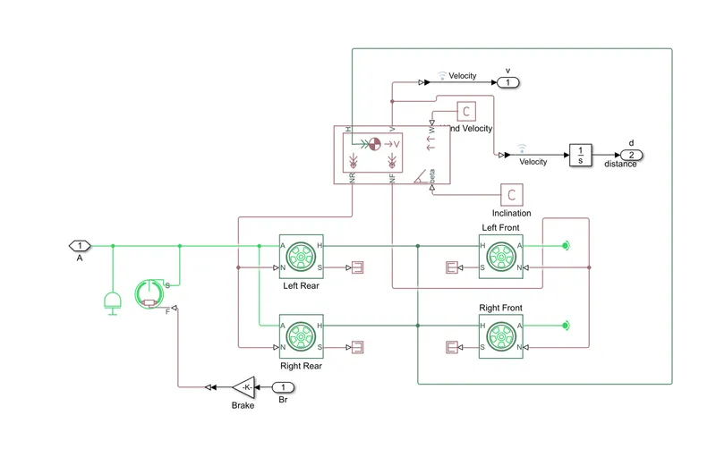
The corresponding vehicle specification are fed into the model, and simulated. For the simulation the inputs includes the Brake input, Throttle input and the CVT Ratio. The inputs are given using a signal builder. This simulates a particular driving scenario.
Inputs :
Brake and Throttle input :
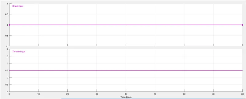
The brake input is zero, and the throttle input is 0.5 from 0 to 80 seconds.
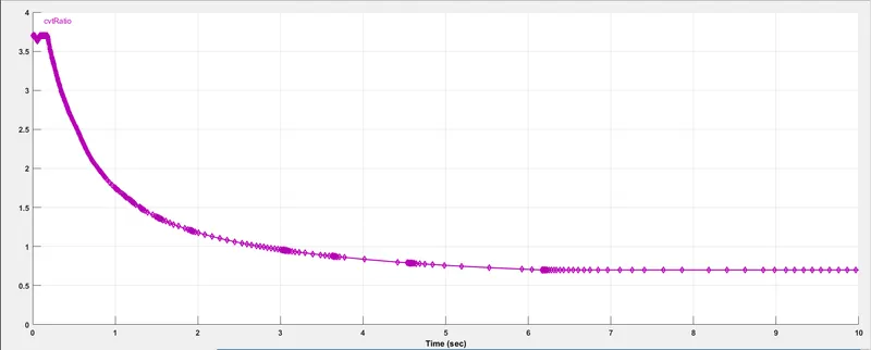
CVT Ratio : A predetermined value of CVT ratio for the simulation is given through a signal builder. The ratio is variable from 0 to 10 seconds, then from 10 to 80 seconds, the ratio is kept constant.
Outputs :
The simulation is performed for 80 seconds. The outputs measured in this simulation includes the Vehicle speed, Distance travelled, Primary and Secondary pulley shaft speeds. The output plots are as follows :
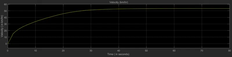
Vehicle speed : It is noted that as the throttle is kept constant, the velocity increases to a limit and then saturates. As we increase the throttle more, the velocity of the vehicle will also increase .
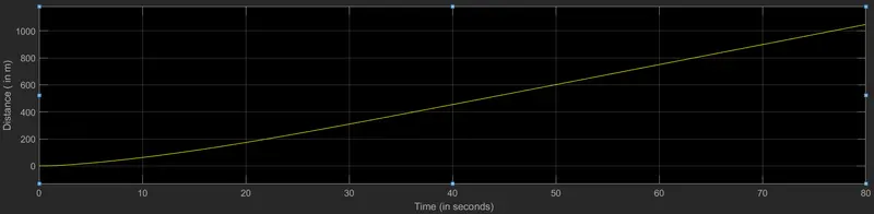
Distance travelled : The distance is a scalar property and hence keeps increasing.
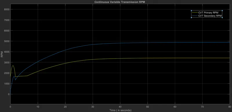
CVT primary and secondary shaft speeds : Depending on the CVT ratio and the engine crankshaft speed, the primary and secondary pulley speeds vary accordingly. It is observed in the input CVT ratio is greater than one until around 3 seconds, after which the CVT ratio reduces below one. The result of this is indicated in the following plot, wherein for the initial 3 seconds, the primary RPM is higher, while the secondary RPM is greater after the initial 3 seconds. Since the variable gear ratio is given only for the initial 10 seoncds, after 10 seconds, the CVT behaves as a constant gear ratio transmission. This is also observed, as both the plot become almost parallel to each other after the 10 seconds.
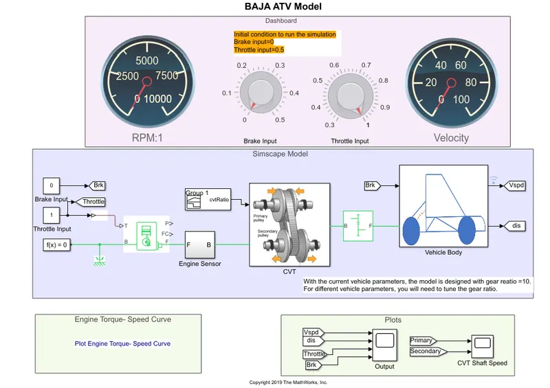
The next variation of the model is with a dashboard, which enables the simulator to manually change the input brake and throttle inputs. In this model, the CVT ratio is kept the same. The brake and throttle inputs are varied, and the corresponding outputs are observed.
Reference : https://in.mathworks.com/matlabcentral/fileexchange/70576-baja-all-terrain-vehicle-atv-model.
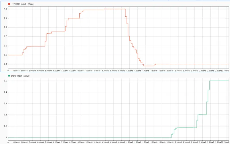
The CVT ratio input remains the same. The model is simulated till 'inf', and the throttle and brake inputs are modified in real-time. All the other vehicle parameters are maintained the same. Corresponding output plots are as follows :
Throttle and Brake Inputs :
Outputs :
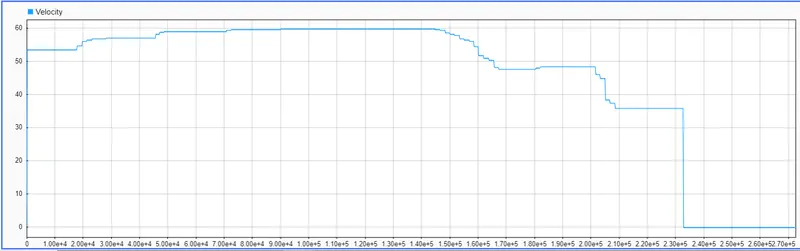
Vehicle Speed: It is observed that as the throttle is increased, the vehicle speed also increases, and as the throttle is decreased the vehicle speed reduces. Likewise, when the brake input is applied, the vehicle speed reduces, and at around the brake input of 0.15, the vehicle speed comes to zero.
CVT - Primary and Secondary Pulley speeds : The trend is similar to the vehicle speed. The reason for the secondary pulley is because, it is connected to the drive shaft, and hence directly is related to the vehicle speed. On the other hand, the primary pulley trend is also similar because the CVT ratio given is only variable for the initial 10 seconds, and then remaines constant at 0.7, the entire system starts to work as a constant gear ratio transmission.
To make the model mode realistic, the CVT ratio is varied according to the speed of the vehicle.
Model 2: In the above model, random values of CVT Ratio was given as input to the model, and the vehicle performance was observed. However, this is not the case in an actual situation (not realistic) , as the CVT ratio is depended on the vehicle velocity. In this model, the CVT ratio is given as a function of the vehicle speed, which is a feedback signal. The model 1 is simulated, the data is logged and the relation between the two parameters is determined.
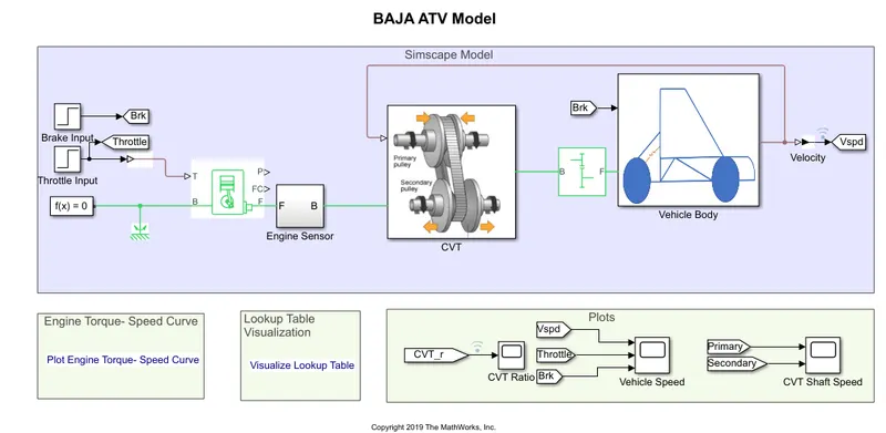
Reference : https://in.mathworks.com/matlabcentral/fileexchange/70576-baja-all-terrain-vehicle-atv-model.
Lookup-Table : A lookup table is an array of data that maps input values to output values, thereby approximating a mathematical function.Given input values, Simulink performs a “lookup” operation to retrieve the corresponding output values from the table. If the lookup table does not define the input values, the block estimates the output values based on nearby table values. The following plot data points is fed into the lookup table. The relation between the CVT ratio and the Vehicle speed, is given through a lookup table, as shown below :
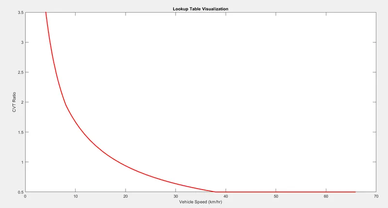
It is observed that the CVT ratio is 3.5 until 4 km/hr. From 4km/hr to 37.5 km/hr, the CVT ratio is variable as shown above. Beyond 37.5 km/hr, the CVT ratio is held constant at 0.5 value. The model is simulated for 200 seconds. The inputs of throttle and brakes are as follows :
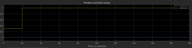
The brake input is 0 throughout the simulation. The throttle input is 0.3 from 0 to 20 seconds, and further increases to to 1 from 20 to 200 seconds, in the simulation.
Outputs :
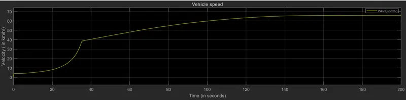
Vehicle speed: One distinctive observation compared to the open-loop model, is that the vehicle speed doesnt varied proportionally to the throttle input, because now that there is a feedback signal, the vehicle speed is dependent on the throttle input and the CVT ratio at the current vehicle speed. The behaviour is more realistic compared to the open-loop model.
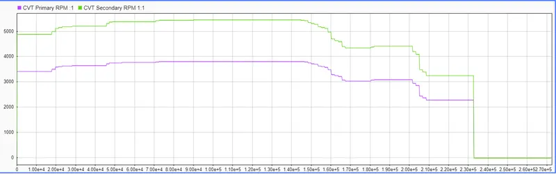
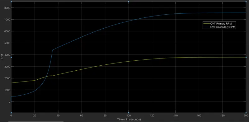
CVT primary and secondary shaft speeds : The secondary pulley RPM has a similar trend as the final vehicle speed.
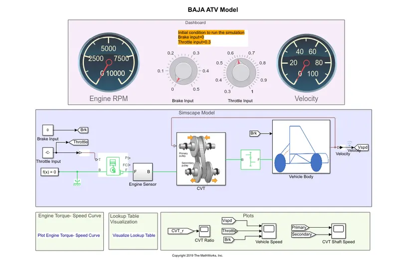
The model 2 is also modeled using the dashboard, where the inputs of throttle and brake can be varied in real-time. The same is simulated, and then the outputs are observed. The model is as follows :
reference : https://in.mathworks.com/matlabcentral/fileexchange/70576-baja-all-terrain-vehicle-atv-model.
The inputs of throttle and brake are given in real-time, and the outputs are observed. The simulation time is kept at 'inf'. The throttle and brake inputs are as follows in the simulation.
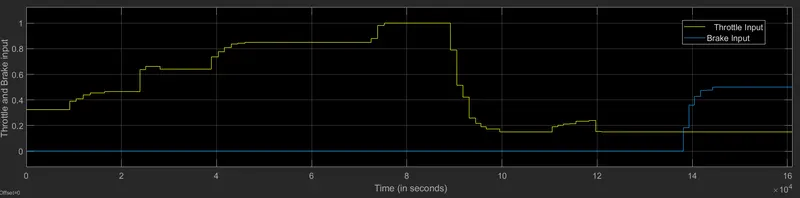
The throttle values in the model is modified to accomodate a minimum value of throttle to be 0.15. Because, at 0.3 input, the speed is 40km/hr, at and beyond which the effect of CVT ratio is constant. To observe the effect of CVT ratio changing, the default throttle input minimum value can be changed from 0.3 to 0.15 (to obtain vehicle speeds below 37.5km/hr).
Outputs:
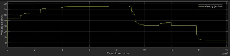
Vehicle speed : The trend is similar to the throttle input.
CVT primary and secondary pulley speed :
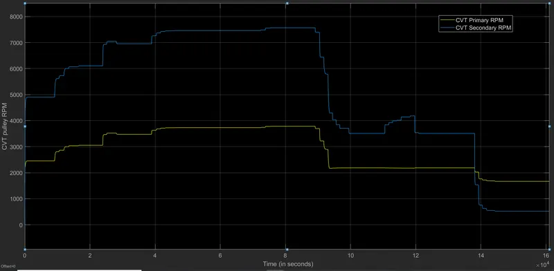
It is observed that when the speed drop below 37.5km/hr, the effect of varying gear ratio of CVT is witnessed. Above that the CVT ratio is constant (0.7). In an actual scenario, the CVT pulley cones movement is controlled using a hydraulic actuators. The main aim of these actuators being controlled using a control system logic, so that the CVT ratio is modified every instant to make sure the engine operating point is within the efficient zone ( area where the fuel consumption in minimum), irrespective of the vehicle output speed. For example, for a given vehicle speed demand and throttle demand, the CVT ratio is modified and estimated at which ratio, the engine operating point is in the efficient region, and accordingly that ratio is selected for running.
References :
Model : https://in.mathworks.com/matlabcentral/fileexchange/70576-baja-all-terrain-vehicle-atv-model.
Mathworks - Improving your Racecar development video series - Modeling of a continuous Variable Transmission (CVT) BAJA All-terrain Vehicle (ATV).
Mathworks - MATLAB and Simulink Documentation help