Project

Simulink for machanical and electrical engineers- project

1. Aim

To study and analyze and make a detailed report on BAJA All Terrain Vehicle (AN) model using Simulink & compare between its different modes. 

2. Objective

Prepare a technical report explaining the model properties & comments on the results.

3. Theory

In Australia, New Zealand, South Africa, portions of Canada, India, and the United States, an all-terrain vehicle, or ATN, is generally referred to as a four-wheeler. Because of their speed and small footprint, they are often utilised in agriculture. According to the American National Standards Institute (ANSI), an all-terrain vehicle (ATV), also known as a light utility vehicle (LUV), a quad bike, or simply a quad, is a vehicle that travels on low-pressure tyres and has a seat that is straddled by the operator, as well as handlebars for steering control. It is built to tackle a broader range of terrain than most other vehicles, as the name indicates. Although it is permissible on the road in certain nations, it is not lawful in most states, territories, or provinces of Australia, the United States, or Canada. ATVs are meant for use by a single operator, according to the current ANSI definition, while other businesses have built ATVs for use by the operator and one passenger. These ATVs are known as tandem ATVs. The rider sits on and controls these vehicles similarly to a motorbike, but the additional wheels provide more stability at slower speeds. Although most have three or four wheels, six-wheel variants are available for particular needs. To differentiate the classifications of vehicles, multiple-user analogues with side-by-side seating are referred to as utility terrain vehicles (UTVs) or side-by-sides. Both classes feature comparable powertrain components.

Baja SAE

The Society of Automotive Engineers International hosts the Baja SAE Collegiate Design Series competition (SAE International). Teams of university students from all around the world design and manufacture miniature off-road vehicles. The engines in all of the automobiles are the same. As of 2018, the engine was a stock Briggs & Stratton Model 19 Vanguard engine with a displacement of 305cc and a power output of around 10 horsepower (7.5 kW). Baja SAE racing's purpose is to develop, manufacture, and race off-road cars that can resist the toughest conditions of rugged terrain. The cars used in Baja SAE racing resemble dune buggies in appearance. Prior to 2007, the tournaments were known as "Mini Baja."

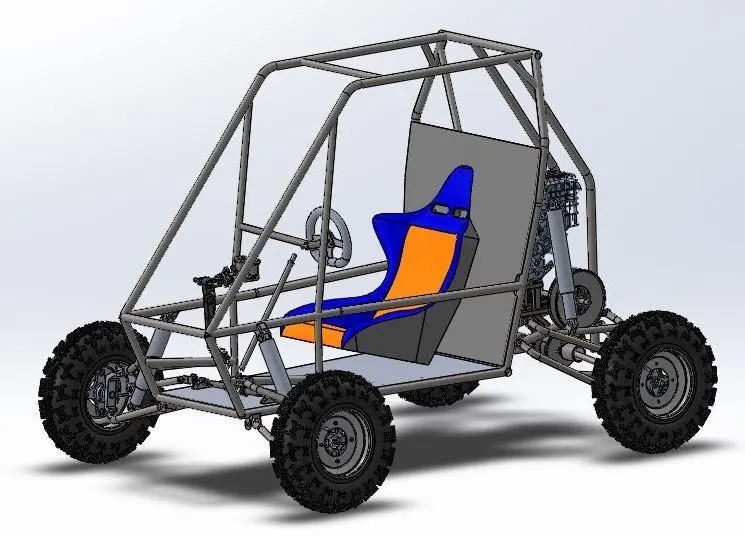
Figure 1: Baja SAE

Simulink ATV models

BAJA ATV model

 

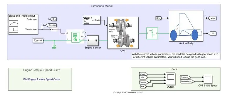
Figure 2: BAJA ATV model in simulink

Simulation blocks used in this model is as below

• Signal Builder — With the Signal Builder block, you may construct interchangeable groups of simple linear signal sources and integrate them in a model.
• Goto — The Goto block sends its input to the equivalent from block. The input might be a signal with real or complex values, or a vector with any data type. The From and Goto blocks let you to send a signal from one block to another without physically joining them.
• Simulink PS Converter — Converts the Simulink input signal to a Physical Signal
• Generic Engine — a system-level model of spark-ignition and diesel engines that may be used when just the fundamental characteristics are available in the early phases of modelling.
• Solver Configuration – Before you can start the simulation, you must provide the solver settings that your model requires.
• Mechanical Rotational Reference—For all mechanical rotational ports, the Mechanical Rotational Reference block serves as a reference point, or frames.
• Engine Sensor — This is a Subsystem model that includes the following simulation blocks and their functions:

 

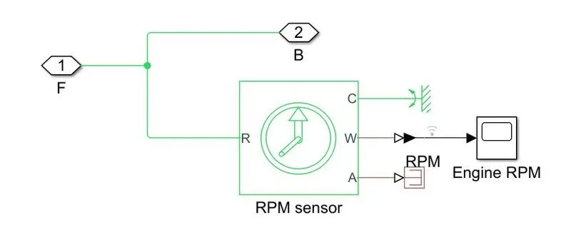
Figure 3: engine sensor

• Ideal Rotational Motion Sensor — The Ideal Rotational Motion Sensor block is a device that translates an across variable sensed between two mechanical rotational nodes into a control signal proportional to angular velocity or inclination.
• Mechanical rotational Reference — All mechanical rotational ports have a reference point, or frame, represented by the Mechanical Rotational Reference block.
• PS-Simulink Converter—  converts the input Physical Signal to a Simulink output signal.
• PS terminator —  this block is use to terminate physical signal outputs.

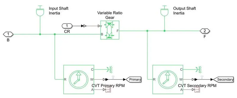
Figure 4: CVT model

• Ideal Rotational Motion Sensor— The Ideal Rotational Motion Sensor block is a device that translates an across variable sensed between two mechanical rotational nodes into a control signal proportional to angular velocity or angle.
• Variable Ratio Transmission — a variable ratio gearbox, such as a mechanical belt CVT, an electric transmission, or a hydraulic transmission.
• Goto — the Goto block sends its data to the From blocks. The input might be a signal with real or complex values, or a vector with any data type. You can send a signal from one block to another using the From and Goto blocks without actually joining them.
• PS-Simulink Converter—  converts the input Physical Signal to a Simulink output signal.
• Inertial — the block represents an ideal mechanical rotational inertia.
• Simple gear - it represented simple gear ratio.

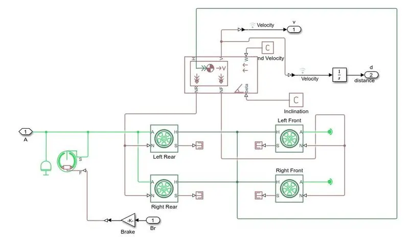
Figure 4: vehicle body

CVT — Vehicle Body It's a Subsystem model made up of the following simulation blocks, each of which serves a different purpose:

• Double Shoe Brake — Represents a brake with two pivoted stiff shoes mounted symmetrically inside or outside a drum and controlled by a single actuator. The shoes exert friction torque on a shaft linked to the drum as a result of the actuator force.
• Gain — Element-wise gain (y = K.*u) or matrix gain (y = k*u or y = uK).
• Tyre — indicates a highway tire's longitudinal behaviour as defined by the tyre Magic Formula.
• PS terminator — This block is used to terminate the outputs of physical signals.
• Vehicle Body — reflects the longitudinal motion of a two-axle vehicle body. Due to acceleration and road profile, the block accounts for body mass, aerodynamic drag, road gradient, and weight distribution between axles.
• PS Constant — this block makes a physical signal constant.
• Integrator — The value of the integral of its input signal with respect to time is output by the Integrator block.
• From — The block takes a signal from a matching Goto block and then outputs it. The output data type is the same as the Goto block's input data type. You can send a signal from one block to another using the From and Goto blocks without actually joining them.
• Scope- this block is use for display the output.

Input variables 

These is the following inputs in the model

The mass input for the inertial at the input shaft and output shaft in the CVT Transmission system is represented by the variables ml, m2. The engine characteristics for the Generic Engine are speedVector and storqueVector, which provide us with the relationship between torque and engine rpm. We used the Signal Builder block to offer throttle and brake input, as well as modify the CVT ratio over time.

 

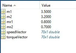
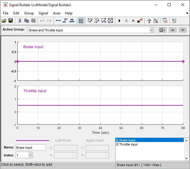
Figure 5: input variables with signal builder block

The mass input for the inertial at the input shaft and output shaft in the CVT Transmission system is represented by the variables ml, m2. The variables'speedVector & storqueVector* are Generic Engine engine characteristics that provide us with the relationship between torque and rpm. We used the Signal Builder block to offer throttle and brake input, as well as modify the CVT ratio over time.

Workflow of the model

The starting condition of the engine block is already defined based on the engine characteristics we know, and the throttle input causes the engine to adjust its speed, torque, and other factors. The variables'speedVector & itorqueVector' are used to give engine parameters for this model. It offers the rpm, torque, and other characteristics based on the engine parameters after receiving the throttle input. The Generic Engine's output passes through the engine sensor block, which records the engine's rpm during the simulation, before being forwarded to the CVT transmission. After going via the basic gear block, which operates as a differential gearbox, the signal from the CVT block was then sent to the vehicle body (tires). The car body block requires two inputs: one from the engine, which is obtained using a basic gear block, and the other from the brake. The input engine signal from the basic gear is delivered to both rear wheels of the vehicle body, since the model is based on a two wheel drive automobile. Because the shafts have rotational inertia, it is coupled to the engine input signal before reaching the tyre. The other input brake is sent to the Double Shoe Brake block, but not before it travels through the gain block, which works as an intensifier for the brake input, or in other words, it multiplies the input force; in this case, the gain factor is 1000. The output from the double shoe brake block is connected to the engine input signal before it reaches the tyre because the brakes are indirectly connected to the input power of the wheels. Another vehicle body block (inside the main system's vehicle body block) accounts for body mass, aerodynamic drag, road incline, and weight distribution between axles due to acceleration and road profile, and distributes the normal forces on the tyres accordingly using the vehicle dynamics data provided to the block. The vehicle's velocity is also obtained as an output from the vehicle body block. The distance travelled by the vehicle is calculated from the velocity signal as it passes through the integrator block. Finally, we have the simulation results in three scope data sets, one with engine rpm, another with the rpm of the primary and secondary shafts of the CVT transmission, and the third with the vehicle's velocity, distance, throttle, and brake values. 

Output Results

Simulation runtime is 200 sec. The engine's initial velocity and rpm is set to 1750 rpm, and as the throttle value is kept constant, the engine's rpm adjusts correspondingly. And, because the throttle setting remains constant during the simulation, the engine rpm remains constant after a specific period of time. Because the primary shaft is connected to the engine, the primary shaft rpm appears to be the same as the engine rpm. However, due to inertia and other reasons, the primary shaft rpm will not be the same as the engine rpm, and some losses will occur. As a result, the primary shaft will not be identical to the engine, but will have similar rpm after accounting for some losses. The secondary shaft speed is then determined by the CVT ratio.

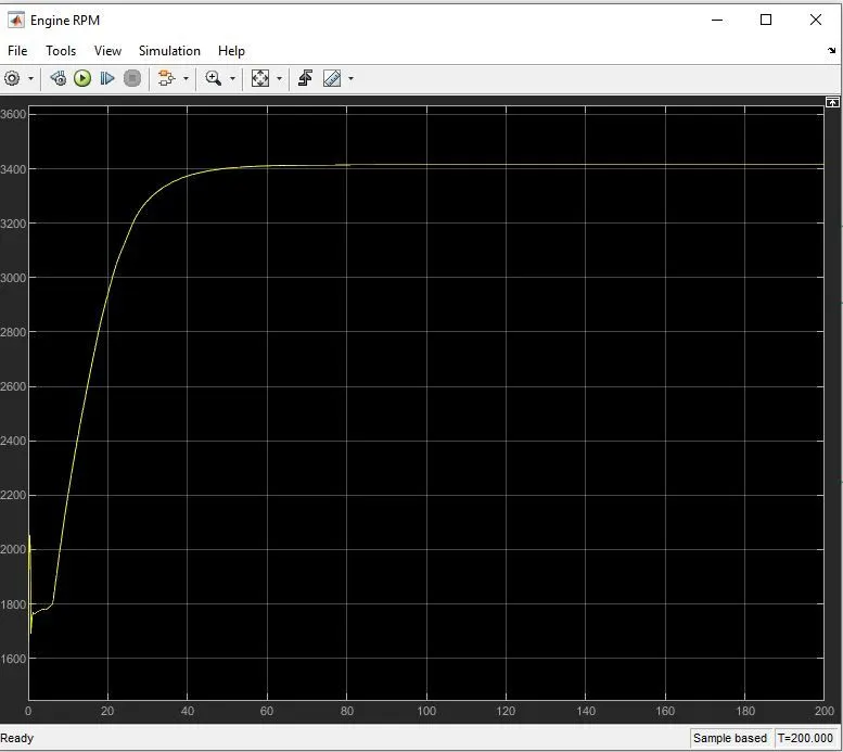
Figure 6: output of engine RPM

We can check that the Throttle and Brake values remain constant throughout the experiment. Initially, the vehicle's velocity is rapidly increased, but after a certain point, when the engine reaches its constant rpm, the vehicle's velocity becomes constant. Integration of velocity provides us the distance travelled by vehicle, as we all know. As a result, the distance travelled seems to be a parabolic curve during the initial simulation time. The distance travelled becomes a straight line as velocity becomes constant.

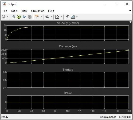
Figure 7: output of various parameters

 

 

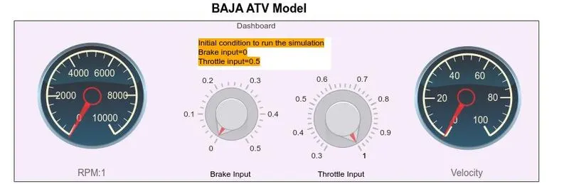
Figure 8: dashboard of BAJA ATV

Dashboard of BAJA ATV model 

This model is the dashboard from the previous model, with the exception that we may alter the throttle and brake values while the simulation is running and then watch the outcomes. The simulation model for the BAJA ATV Model with dashboard is shown in the figure.

• Circular Gauge – A customizable gauge that displays an input value.
  Set a value using the knob to fine-tune parameters or variables. 
• Fixed — Returns the value supplied by the 'Constant value' parameter as a constant.
• Generic Engine — This is a system-level model of spark-ignition and diesel engines that may be used in the early phases of modelling when just the fundamental characteristics are known.
• Solver Configuration —The Solver Configuration section specifies the solver settings that your model requires before the simulation can begin.
• Mechanical Rotational Reference — The Mechanical Rotational Reference block serves as a frame or reference point for all mechanical rotational ports.
• Engine Sensor— this is a Subsystem model made up of the following simulation blocks, each of which serves a specific purpose:

Moreover other blocks like engine sensor, CVT and vehicle body has been described earlier with figure of each block. Simulink blocks used in those sub system also have been described.

Inputs of the model

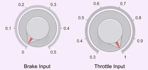
Figure 9: brake and throttle input

The knob block is used to give throttle and brake input while the simulation is running, and its limitations are displayed on the knob. The engine block's starting condition is already established based on the engine parameters we know, and then the engine's speed, torque, and other characteristics are changed based on the throttle input. The engine parameters for this model are supplied through the variables speedVector and 'torque'. Vector: The user provides the throttle and brake inputs using user interface knob blocks, which allow the user to modify the throttle and brake inputs while the simulation is running. After the system has received the throttle and braking inputs. Depending on the engine specifications, the engine block delivers the rpm, torque, and other elements. The output of the Generic Engine is routed to the engine sensor block, which records the engine's rpm during simulation, and then to the CVT Transmission. The CVT block receives two inputs: one from the engine and the other from the signal builder block, which calculates the CVT ratio. There are two ideal rotational sensor blocks and two inertia blocks for input and output shafts, respectively, in the CVT block, and then there's the Variable Ratio Gear, which adjusts its gear ratio during the simulation based on the CVT ratio. The signal from the CVT block was now sent to the basic gear block, which operates as a differential gearbox, before being routed to the car body means tires. The car body block requires two inputs: one from the engine, which is obtained via the basic gear block, and the other from the brake. Because our model is based on a TWD (Two Wheel Drive) vehicle, the input engine signal from the basic gear is sent to both rear wheels of the vehicle body. Because the shafts will have rotational inertia, it is then coupled to the engine input signal before reaching the tyre. The other input brake is delivered to the Double Shoe Brake block, but before it gets there, it travels via the gain block, which functions as an intensifier for the brake input, in other words, it multiplies the input force, in this case by 1000. Because the brakes are indirectly connected to the wheel's input power, the output from the double shoe brake block is connected to the engine input signal before it reaches the tyre. On the primary system, there is another vehicle body block inside the vehicle body block that accounts for body mass. Aerodynamic drag, road gradient, and weight distribution between axles owing to acceleration and road profile are among factors that the block considers while distributing normal forces on the tyres. We also obtain the car's velocity as an output from the vehicle body block. The distance travelled by the vehicle is provided by the velocity signal when it passes through the integrator block. Finally, we have the simulation results in three scope data, one with engine rpm, another with the rpm of the primary and secondary shafts of the CVT transmission, and the third with the vehicle's velocity, distance, throttle, and brake values.

Results with different cases 

Case 1

when brake=0 and throttle= 0.5

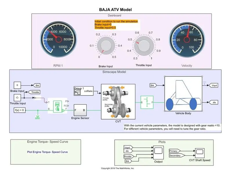
Figure 10: Case 1

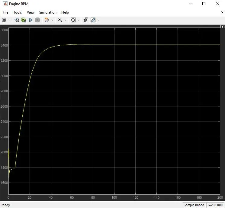
Figure 11: engine RPM

The engine's initial velocity/rpm is defined at 1750 rpm, and when the throttle value is constant input, the engine's rpm varies correspondingly. Because the throttle setting remains constant during the simulation, the engine rpm becomes constant after a specific period of time.

 

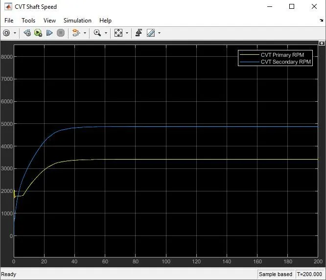
Figure 12: CVT shaft speed

Because the primary shaft is connected to the engine, its rpm seems to be the same as the engine rpm; nevertheless, owing to inertia and other considerations, the primary shaft rpm will not be the same as the engine rpm and will have some losses. As a result, the primary shaft will not be the same as the engine, but will have similar rpm after accounting for certain losses. The secondary shaft speed is determined by the CVT ratio.

We can see that the Throttle and Brake values remain consistent throughout the experiment. Initially, the vehicle's velocity is rapidly increased, and then, at a certain point, when the engine achieves its constant rpm, the vehicle's velocity becomes constant. Integration of velocity, as we know, provides us the distance travelled by vehicle. When a result, the distance travelled seems to be a parabolic curve during the first simulation time, and subsequently becomes a straight line as velocity becomes constant.

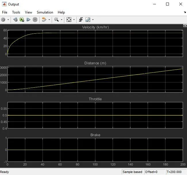
Figure 13: output of various parameters

Case 2

Brake=0 throttle=varying

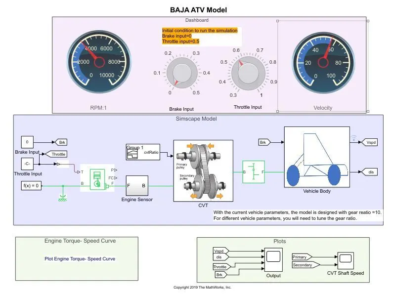
Figure: 14: case 2

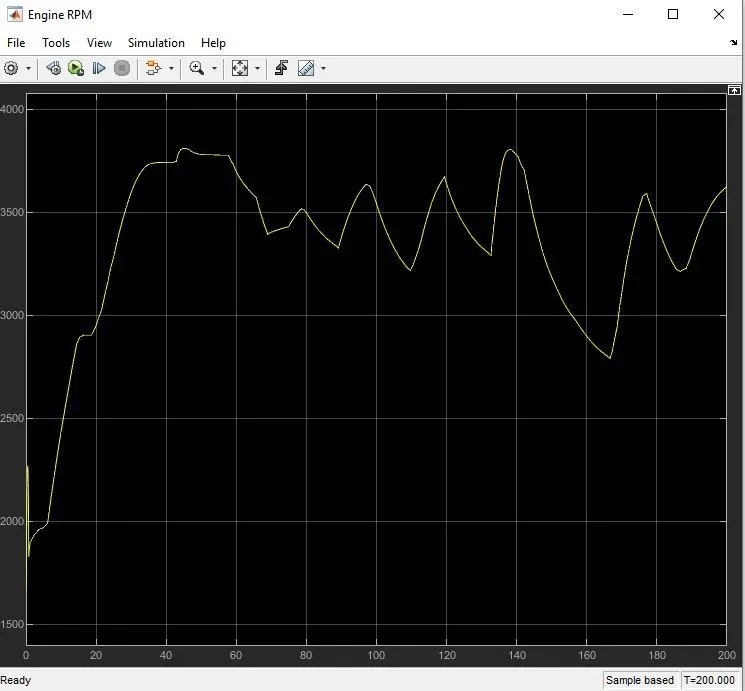
Figure 15: output of Engine RPM

The engine's beginning velocity/rpm is set at 1750 rpm, and the brake value is constant. Initially. For a short period of time, the throttle is held constant until the vehicle's rpm/velocity begins to stabilise. Then, when we alter the throttle value, we notice ups and downs in the engine's rpm. Increasing the throttle raises the engine's rpm and vice versa. Following that, we see that increasing the throttle fast raises the rpm and generates a sharp slope line/curve on the graph. However, while lowering the throttle. The engine's rpm progressively decreases, forming a curve line on the graph.

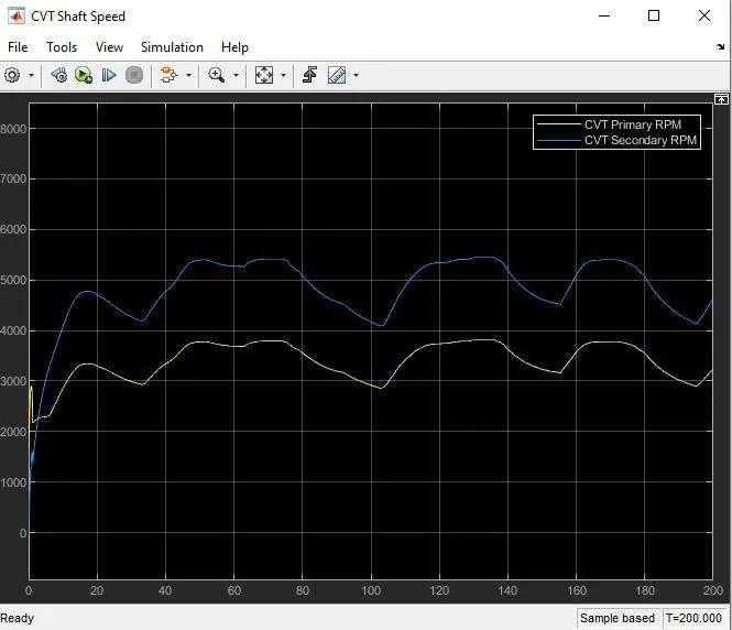
Figure 16: CVT shaft speed

Because the primary shaft is connected to the engine, its rpm seems to be the same as the engine rpm; nevertheless, owing to inertia and other considerations, the primary shaft rpm will not be the same as the engine rpm and will have some losses. As a result, the primary shaft will not be the same as the engine, but will have similar rpm after accounting for certain losses. And the secondary shaft speed is determined by the CVT ratio.

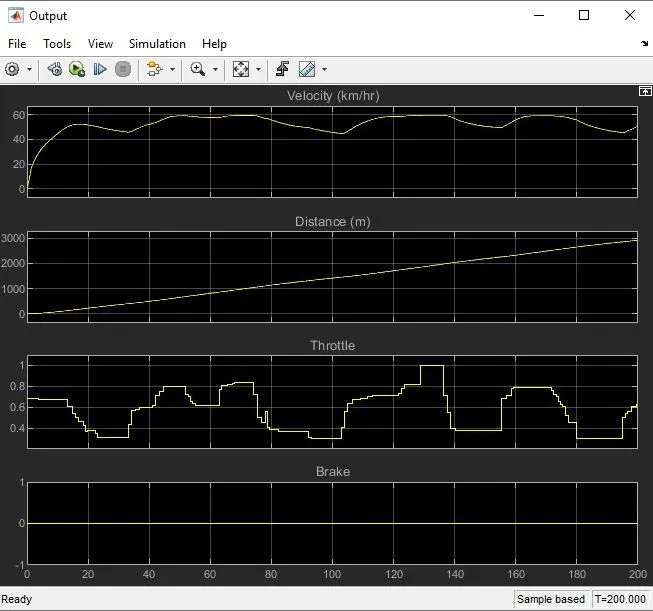
Figure 17: output of various parameters

We can see that the brake remains constant throughout the experiment. The throttle line indicates how much throttle is applied and when it is applied, as well as the duration of the applied throttle. Here we can plainly see the influence of the applied throttle value on the velocity of the car; as the throttle value grows, the velocity of the vehicle begins to increase fast, but as the throttle value falls, the velocity of the vehicle decreases slowly. Depending on the engine's output power. We can see that velocity is controlled by throttle in the same way as the engine is, and the velocity graph looks identical to the engine rpm graph, except multiplied by CVT and simple gear. It was also harmed as a result of other vehicle dynamic losses. Integration of velocity, as we know, provides us the distance travelled by vehicle. When a result, the distance travelled seems to be a parabolic curve during the first simulation time, and subsequently becomes a straight line as velocity becomes constant.

case 3

Brake= varing thorottle= 0.6

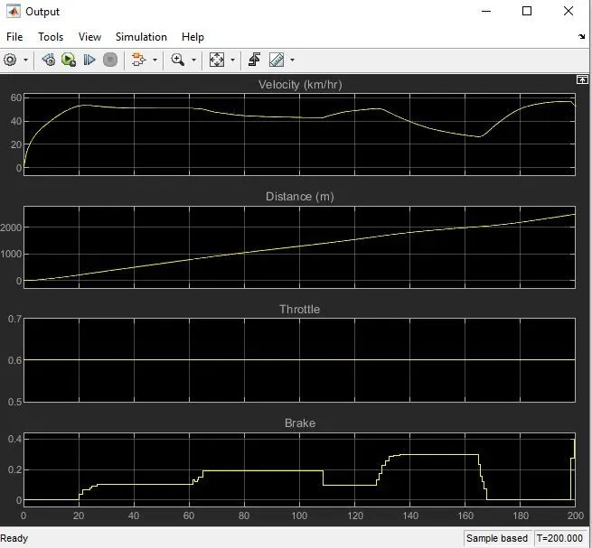
Figure 18: output of various parameters

We can see that the throttle remains constant throughout the experiment. The brake line indicates how much brake is applied when it is applied, as well as the length of the brake application. Here, we can plainly see the effect of the applied brake value on the vehicle's velocity; as the brake value increases, the velocity begins to drop. However, when we apply break at less than 0.12 or 0.1 value, velocity continues to increase but at a slower pace, and when we apply break at greater than 0.12 or 0.1 value, velocity begins to decrease at a rate dependent on the amount of applied brake. Depending on the engine's output power. We can see that brakes effect velocity in the same way that the engine does. And the velocity graph resembles the engine rpm graph, except that it has been multiplied by CVT and simple gear, as well as modified by other vehicle dynamic losses. Integration of velocity, as we know, provides us the distance travelled by vehicle. When a result, the distance travelled seems to be a parabolic curve during the first simulation time, and subsequently becomes a straight line as velocity becomes constant.

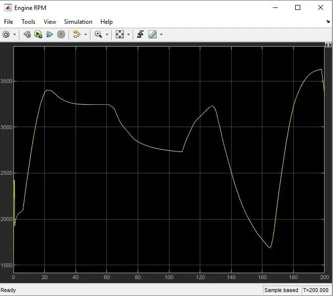
Figure 19: Engine RPM

The engine's beginning velocity/rpm is set at 1850 rpm, and the throttle value remains constant. We can see from the video that the throttle value stays constant for the first 20 seconds of the simulation and no brake is applied, therefore the engine rpm is controlled by the throttle input. The engine rpm begins to fall as we progressively apply the brake, then after 164 seconds, the engine rpm suddenly increases to its peak. The engine rpm decreases faster for high brake values and vice versa depending on the brake value, as we can see in the graph lines.

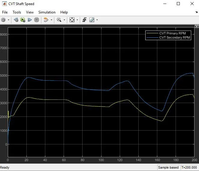
Figure 20: CVT shaft speed

Because the primary shaft is connected to the engine, the primary shaft rpm seems to be the same as the engine rpm. However, owing to inertia and other reasons, the primary shaft rpm will not be the same as the engine rpm, and some losses will occur. As a result, the primary shaft will not be identical to the engine, but will have similar rpm after accounting for certain losses. The secondary shaft speed is then determined by the CVT ratio.

Conclusion

We can clearly see how the car will operate in the given circumstances. It also can be determined that time it takes to reach a specific speed or to totally stop the car. We can also be able to determine the vehicle's maximum speed analysis the curve. The performance of the brake system and the throttle system may also be observed. This model allows us to test the vehicle's performance using the built-in brake and throttle systems.