Project

AIM : TO CARRY OUT A SYSTEM LEVEL SIMULATION OF AN ALL TERRAIN VEHICLE .WE ARE GIVEN THE MODEL ; RUN THE SIMULATION AND DO THE ANALYSIS.

OBJECTIVE : Download the model from the given link, and prepare a technical report explaining the model properties & comments on the results

Introduction :

The image of an All Terrain Vehicle is as give below.

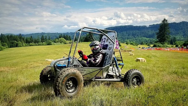
An All Terrain Vehicle ( or ATV ) is a vehicle specially designed to handle almost all types of terrain unlike the other vehicles available in the market. Mostly this ATV will be a single seater vehicle, with low pressure tyres.

Baja SAE being a Collegiate Design series competition is run by the Society of Automotive Engineers International. Teams developed from many colleges from different parts of the world design and build their offroad small vehicles. So here we are asked tostudy the model and prepare the result of the same.

Here the vehicle runs on Continuous variable transmission .

Continuous Variable Transmission is a kind of automatic transmission which allows seamless change through a range of gear ratios.CVT allows to run at the same RPM while cruising in different speeds. CVT doesnt use a clutch pedal .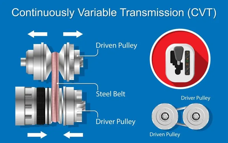

BAJA ALL TERRAIN VEHICLE SIMULATION MODEL :

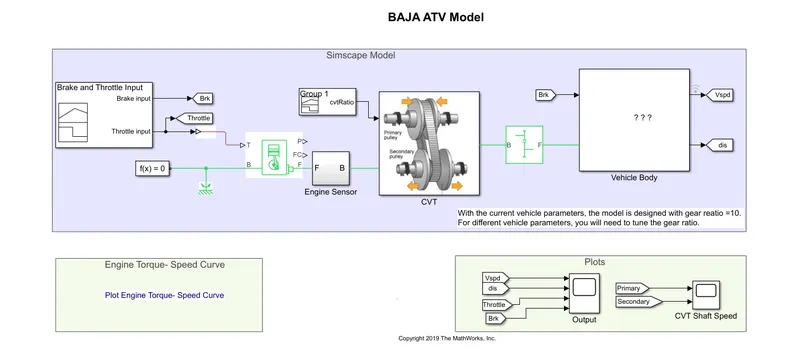
EXPLANATION :

(I ) Signal Block

Lookin at the initial phase of the model we can see a Signal Builder Block , which produces two signals as input to the latter model namely Brake Input and Throttle Input . Signal builder produces the following signal :

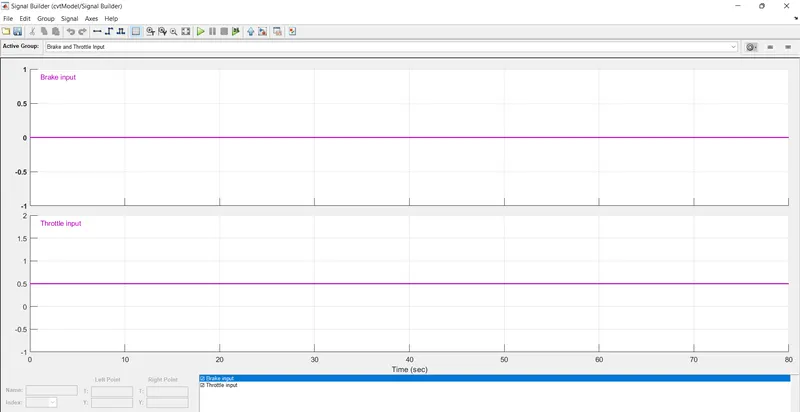
We can infer that the Brake input delivered into the system is a signal with a null value and Throttle Input is of value 0.5 .

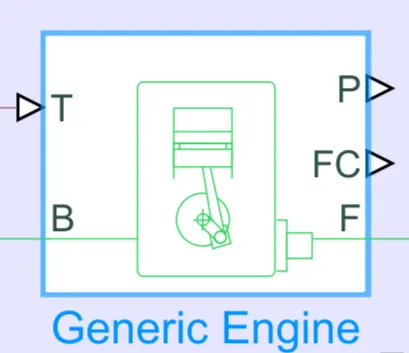
( II ) Generic Engine Block : The output from the signal builder (Throttle Input ) is given to a Generic Engine block , which is used to represent a system level model of a Spark Ignition . This Throttle input 'T' is always fed as a value between 0 & 1 ., which is a representation of percent value of the maximum possible throttle that can be given to the system .The B and F connections are the mechanical rotational conserving ports associated with engine block and engine crankshaft respectively .Connections P & FC are physical signal output ports reporting instantaneous EnginePower and Fule consumption rate respectively. If the engine speed goes less than the Stall speed then the Torque will go to zero. Also if the engine speed goes above the maximum speed then simulation stops and an error message is displayed.

( III ) Engine Sensor : In this subsystem we have an Ideal rotational motion sensor , a PS terminator and a mechanical rotational reference attached to it . The output from the Generic Engine model will be given to an Engine sensor subsystem. The output values from the Generic engine to be given to the CVT is recorded using the sensor block .

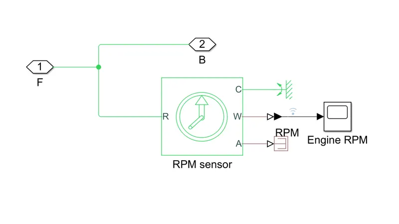
The PORT W of the sensor is connected to a converter and then given to a scope to display the Engine RPM .

(IV) CVT : This block has a subsystem in it , which is used to represent the continuous variable transmission process.

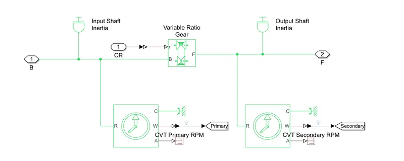
fig . CVT subsystem

Looking at the CVT subsystem we can see the following blocks :

(a) Inertia block : This is used to represent an ideal mechanical rotational inertia. The direction of rotation from the port to the reference point is considered positive direction i.e inertia torque is positive if accelerated in a positive direction . Here we have two inertia blocks , namely ; Input and Output .

(b) Variable gear ratio : It is used to represent a variable speed gearbox .It has an input connection 'r' which define the ratio of input to output angular shaft velocities. Then there are two mechanical rotational conserving ports 'B' & 'F' .

(c) Ideal rotational motion sensor : This block is usedc to measure the angle or angular velocity in a mechanical rotational system .

(d) Mechanical rotational reference and PS Terminator :

CVT Block is the block which accepts input from the CVT gear ratio and the engine parameters and then gives the output to the Wheels( tire block ). A Simple gear block is attached in between both these blocks to transfer the CVT power to the Wheels. The power output from the Simple Gear block is then delivered to the input of the Vehicle block . A scope is also connected so that the Throttle input and Brake input can be seen .

( V ) Vehicle body : The output of this Simple Gear block is then fed to the Vehicle Body subsystem .

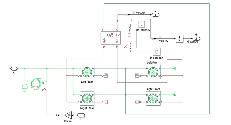fig. Vehicle body subsystem

This block shows the complete Vehicle assembly which shows all the input required to operate the engine . It has the following blocks in it :

(a) Vehicle Body : A two axle vehicle body going in a longitudinal motion is represented by this block .

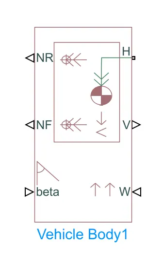
The H port seen here is the Mechanical Translational conserving port which is related to the horizontal motion of the vehicle . The connections V , NF AND NR are used for output ports which are used for Velocity , Front and Rear Normal wheel forces respectively .

Parameters of the vehicle body block is as shown below :

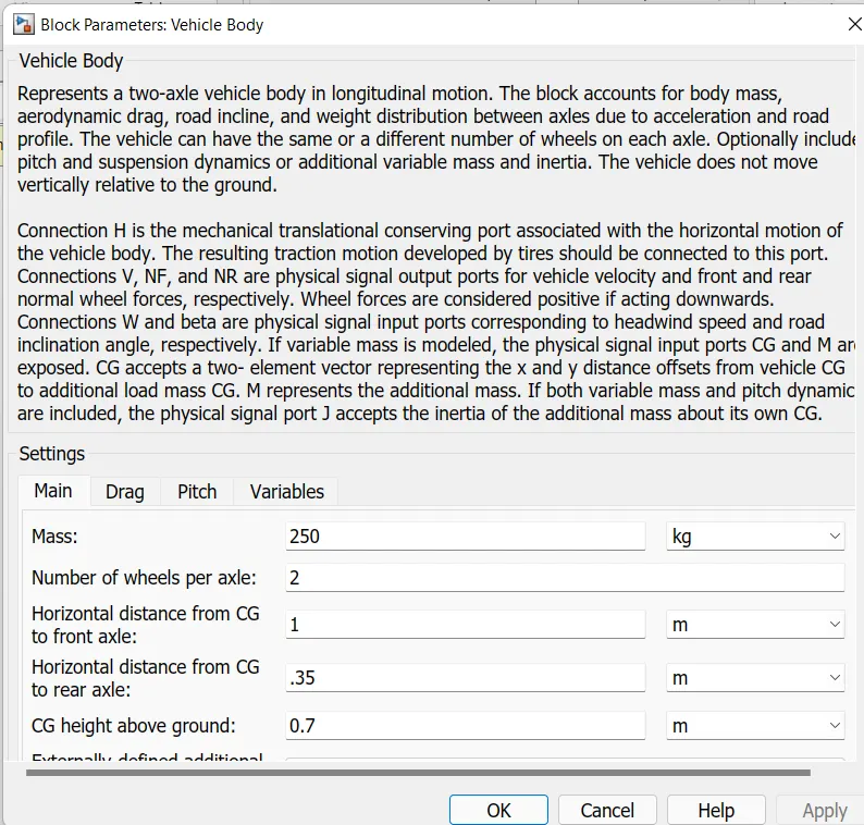
(b)Tire : This block represents the longitudinal behaviour of the tire which is represented by a Magic formula .

(c) Shoe Brake : This block represents the brake of the vehicle which is arranged as two pivoted shoes which is symmetrically placed and operated by an actuator . Following figure represents the parameters of the Shoe brake Block.

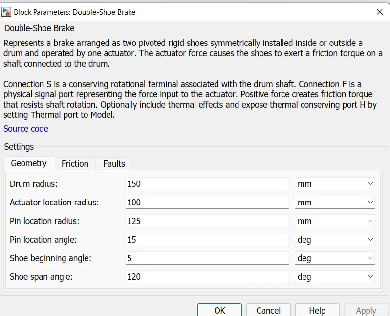
(VI) Solver Configuration : For simulation to run without any flaws we use this block to configure the solver settings .

(VII) Mechanical Reference : Used to represent mechanical rotational reference .

(VIII) GoTo and From block : These blocks are used to pass signals from one another . These passing of signals can be done without any connection between the signals . Here it is attached to the output of the Vehicle body block and the scope block respectively . The perfromance curve can be seen from this .

(IX) Scope : Used to display the signals .

(2) ATV MODEL WITH A DASHBOARD :

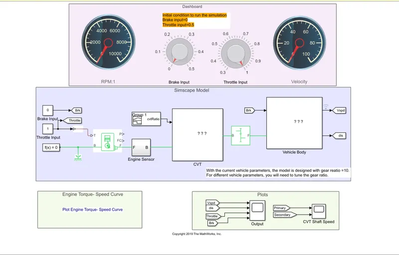
In this model of ATV we dont use a Signal builder as we have done in the revious model , but instead we have used a Circular Gauge Block which plays the role of a Speedometer where values could be displayed from the Input knob. This knob can be used to provide the input values for both Brake and Throttle inputs, by setting the knob as per the required conditions . Everything else are similar in both the ATV models .

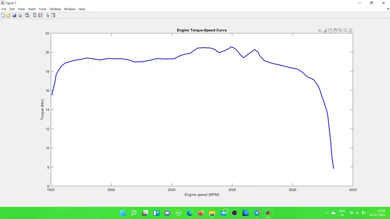
Engine Torque-Speed Curve

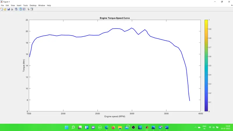
We can observe here that initially the system has a very high torque for the initial pickup .But gradually as Speed increases, we can see that Torque decreases with increasing speed.

ENGINE RPM :

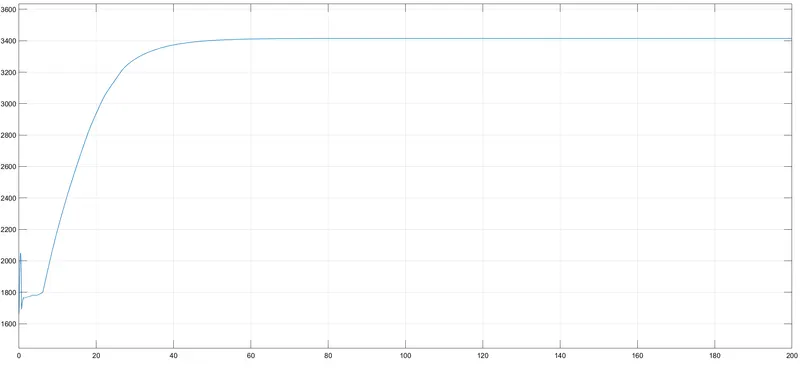
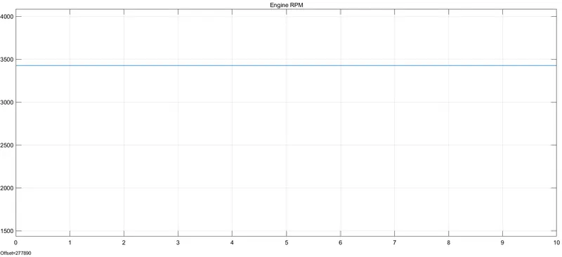
Here we can observe from the above graph that after a gradual increase in the Speed then the speed becomes a constant value later.

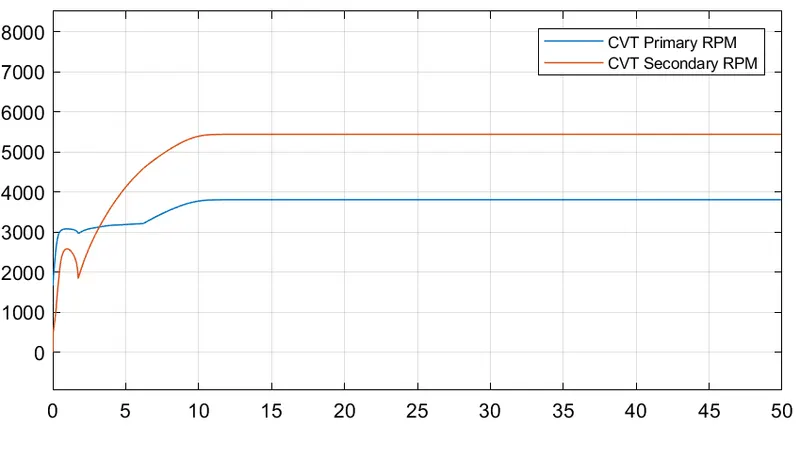
CVT SHAFT SPEED Graph :

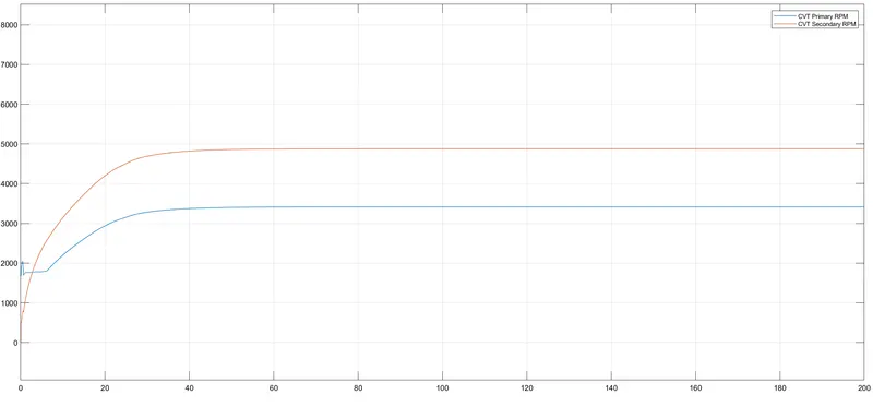
We can see here the CVT Secondary RPM with '0' value and then within a little span of time it rises to a huge value .

PART II : Simulink model of All Terrain Vehicle with a Lookup Table

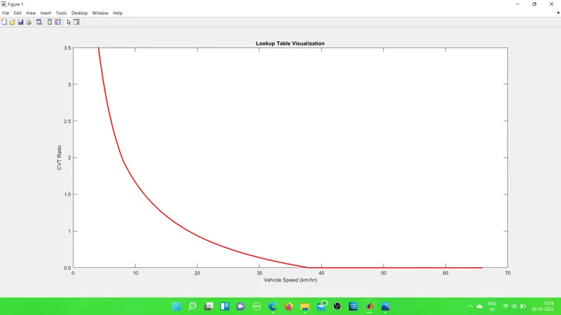
Lookup Table : A lookup table is similar to a mathematical function which maps input values into output values.

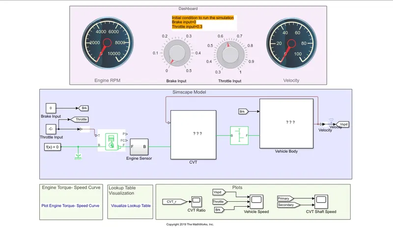
fig . ATV DASHBOARD MODEL WITH LOOKUP TABLE

The only difference here is that we have a Lookup table in this setup.

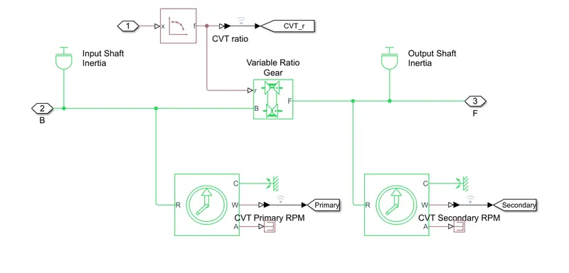
THE CVT will be now as follows :

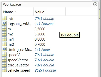
WORKSPACE DETAILS :

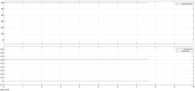
SCOPE OUTPUT :

ENGINE RPM :

Lookup Table visualization :

Engine Torque-Speed graph :

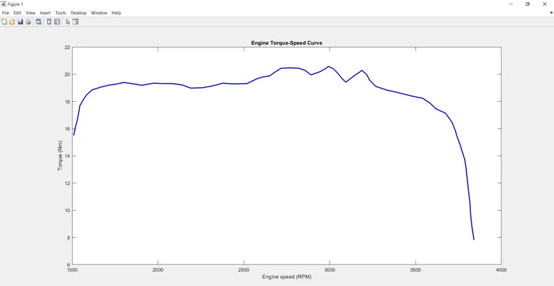
FIG BELOW : CVT SHAFT SPEED CURVE

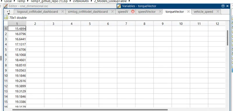
Torque vector :

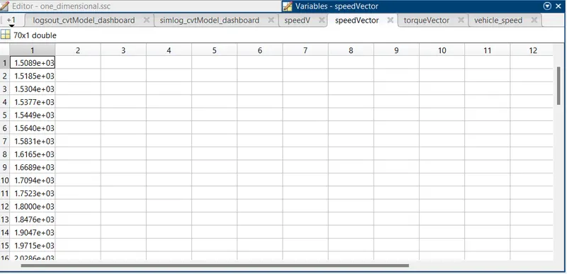
Speed Vector :

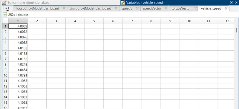
Vehicle speed :

Testing the Model

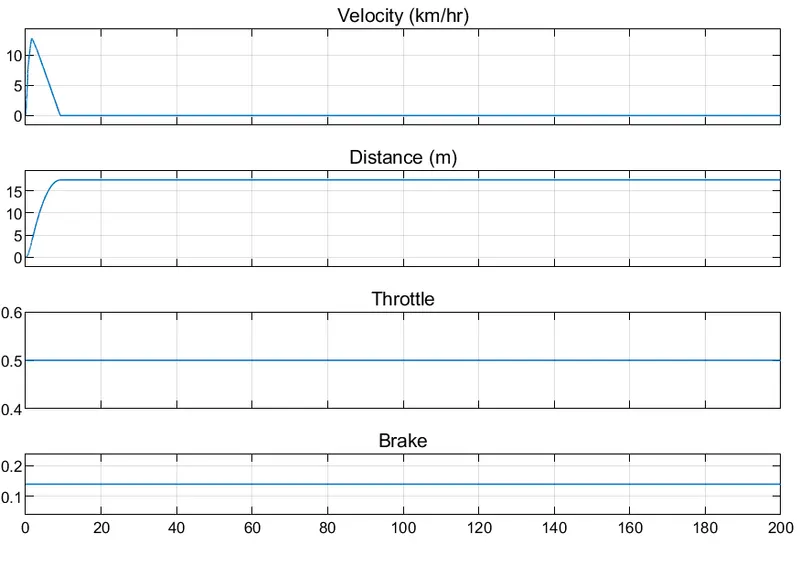
(i) Without a Lookup table and without dashboard :

Brake = 0.14 and throttle = O.5

WE get the following output

.

(ii) Without lookup table with dashboard :

Changing brake = 0.16 and Throttle to 0.95 we get the result as

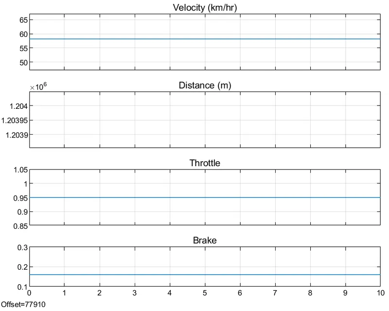
So we can infer from the above graphs that Speed becomes almost constant after a certain interval of time and if the brake is applied then the speed will decrease further .

RESULT :

The complete analysis of the All Terrain Vehicle was done and the study of the same under various conditions were carried out .

All the details were given in the following link .:

https://www.mathworks.com/matlabcentral/fileexchange/70576-baja-all-terrain-vehicle-atv-model