Project
ATV
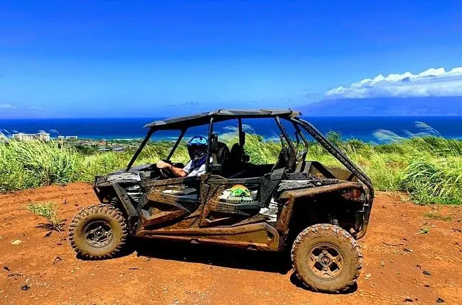
An ATV or all terrrain vehicle is on which has a capability to dodge any road challenge on any road conditions in terms of on and off-road. It has a great suspension travel to provide good damping at the time of nimbling the off-road conditions. Off-road terrain is full of challenges with ups and downs,muddy surface or even water loggings, and to overcome these,an ATV has good ground clearance. It is also fitted with crash guards all over the body to keep the vehicle (body along with engine) and the driver safe from flying stones and Earth. Atv is fitted with a powerful and torquey engine to climb steep slopes or escape the tough terrain. It has a continous variable transmission or variomatic transmission for smooth shifting of gear without efforts so that the rider could only focus on the terrain and not on the vehicle while driving one. They travel on low tire pressure in order to increase the contact patch and gain sufficient grip in loose road conditions.
CVT
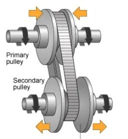
Continous variable transmission is a leverless shifting of gears which is a nothing but a automatic mechanism. In this system, there is no need of shifting gear with increase in the speed. The system automatically shifts form low to high and vice versa depending on the throttle input provided.
Parts
1)pulley- there are two pulleys *)driven and *)driver. Driven pulley is connected to the wheel axle and driver pully is connected to engine output shaft.
2)Push belt- It is made of small steel components in a specific bond design and rotates on the two pulleys. The belt actually couple the two pulleys. Driver pulley is made of two pulley which is meshed with each other. One is fixed and other one is movable. Same is applicable for the driven pulley. The movable pulley on both the driven and driver shaft is hydraulically(oil). controlled and is designed to move in one direction.
Working
The driven and driver pulleys are coupled by the push belt which transfers the torque from the former to the latter. When the throttle is released, the driver pulley which is connected to the output engine shaft, compresses making the belt to reduce the radius of the rotation at the same end. This in turn makes the driven pulley to expand. The belt rotating on this end results in an increased radius of rotation when looked from the side. The output of the this is that the vehicle starts deccelerating. On the other hand, if the throttle is applied then the driver shaft compresses making the belt radius of rotation to increase. This increased belt rotation radius decreases the belt rotation radius at the driven pulley when the this driven pulley expands. But this can be altered in order to get different torque output.
For reverse gear, there is an epicyclic meshed with the driven pulley. Epicyclice gear is made of a centre gear which is Sun gear,many small gears meshed with Sun gear known as planet gears,and the bog gear on the outter side which is called as ring gear. The Sun gear is mounted on the input shaft of the driver pulley. There is a clutch which rigidly connects the Sun and ring gear perfectly. This is always fixed in forward gear motion. But when the reverse gear is shifted, the clutch is released which makes the Sun, Ring gear to rotate in opposite direction with respect to each other with the help of plannetary gears. This in turn, will make the driver pulley to rotate in opposite direction making the vehicle to move in reverse direction.
Benefits
1)Compact engine
2)better efficiency
3)Easier driving experience
Baha is a competition where a nowhere land or and off-road map is selected and the participants have to race against the time to complete the full map and reach the finish line. There are teams with two drivers who switch in between the races in order to take rest and get ready for the next round. The cars have the same engines but the tuning and the parts make it different from each other. The vehciles are made to go through the most harsh conditions in order to win Baja. The cars look similar to a small buggy car.
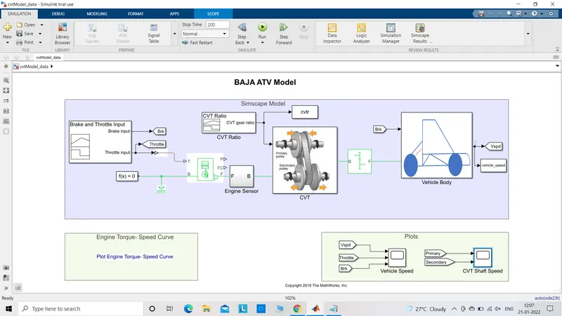
The Atv. model was opened in simulink and the following was observed:-
The model has a dashboard consisting controllers and displays. There is a analog speedometer which has range 0-100km/h. An rpm analog meter with range 0-10000 engine speed in revolution per min. There are two input knobs which is used to input the braking or torque to the vehicle. Initially the brake input is set to 0 and torque to 0.5 to run the simulation.
The corresponding model is the processing model which will be affected by the above inputs. While driving, we apply brake or acceleration which gets processed in the engine unit and then the effect are seen on the whole vehicle which would either slow or speed up depending on the input. This is a simscape model with throttle and brake input taken by the lookup tables prepared in a seperate sheet and then imported to matlab and used here as input values of throttle and brake.To load the file, matlab code is used as shown:-
The graph is the input signal which would be set manually in the signal builder block. It is drawn between the cvt ratio means the difference in the input and output angular speed with respect to each other and vehicle output speed. This is done by using gears of different diameters. In cvt as shown earlier, the region in between the two pulleys is tappered and so different diameters are achieved.
The graph shows that when the car is at rest, the gear ratio is high which means high diameter output and low diameter input. As the vehicle accelerates, the gear ratio gets reduced which means both the gear start to come closer and closer in terms of size when switching from low gear to high. This is same in cvt also, where the diameter of the pulley at driven and driver end come close to each other till the car has reached around 38 km/h and then the car achieves the lowest gear ratio which means it is in the top gear and the speed is increasing and crosses 65km/h. The graph also tells us that the acceleration is less from 5- 15 km/h and then slowly rises after crossing 20km/h.
This is going to be send as input to the engine so an engine block is connected via a simulation-ps block. the output of engine would be observed by the engine sensor. The output would be the engine rpm which would act as an input for variomatic transmission. A signal builder is used to input values to cvt block which is nothing but the speed mentioned earlier.
The cvt is then connected to a simple gear representing the gear meshing of cvt with the axle. Then finally, we have the vehicle body connected to the dispay for observing the the behaviour of the graph.
CVT block is a subsystem and it contains all the blocks which represent primary and secondary pulleys.
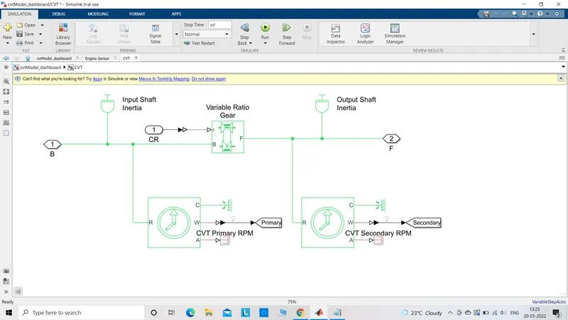
Two shaft inertia blocks are used for both the pulley to represent a real phenomenon. Two rotational source are used to represent the two driver and driven pulleys which are then connected to variomatic gear block to represent cvt transmission.Different gear ratios can be used according to the model which we are making. Here, the simple gear ratio is set to 10.
The vehicle body is also a subsystem and has:-
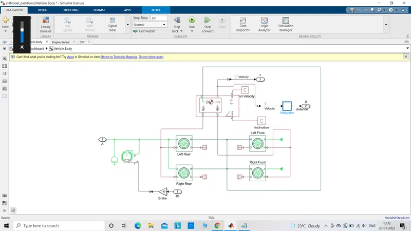
There are 4 wheels with slip values, horizontal movement, axle ,normal force. We have assumed no slip so an ps- eliminator block is used to terminate to close the output port at S. All H are connected and axles A to respective front and rear ones. Axle A is connected to a rotational free end which means it would rotate without any torque. This is done for only the two front wheels. The rear wheels are connected to double shoe brake and rotational inertia blocks is connected to represent a practical scenerio. All normal N are connected. Vehicle body block has normal value for rear and front NR, Nf, wind resistance W,,horizaontal movement H,velocity V and beta if a car is required to move on a gradient. Wind drag and beta are given some values which represents the car is moving on a gradient and is subjected to air drag. This completes the vehicle modeling part.
The 4 models are:-
1)BAJA ATV model without dashboard
2)BAJA ATV model with dashboard
3)BAJA ATV model with look-up table without dashboard
4) BAJA ATV model with look-up table with dashboard
1)Model with signal builder as input without dashboard
The input signal is named as brake and throttle input.
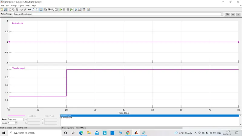
The above signal builder shows that there is no brake input given at all. The total time is 80 secs. Throttle on the other hand is set to 0.3. The car is revved after 20 secs to value 1. The throttle is set to 1 for full 80 secs.
The input to cvt is given in by another signal builder.
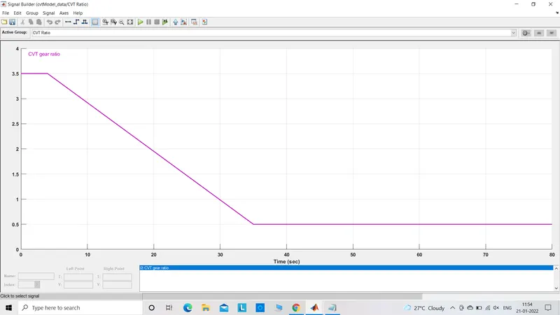
The signal builder shows that the gear ratio remains till the throttle is not given intially for around 4 secs. The cvt gear ratio is 3.5. Then after 4 secs, the throttle is applied and the graphs show a gradual decrease from 3.5 to 0.5 as the gear ratio in order to speed up the vehicle till 35 secs. The ratio remains constant which means that there is either the vehicle has reached the red lining and there is no more further throttle opening possible in order to supply more air-fuel mixture or the car is set to a constant speed somewhere in between for the rest of the time till 80 secs. This is the input to cvt block.
Output graphs
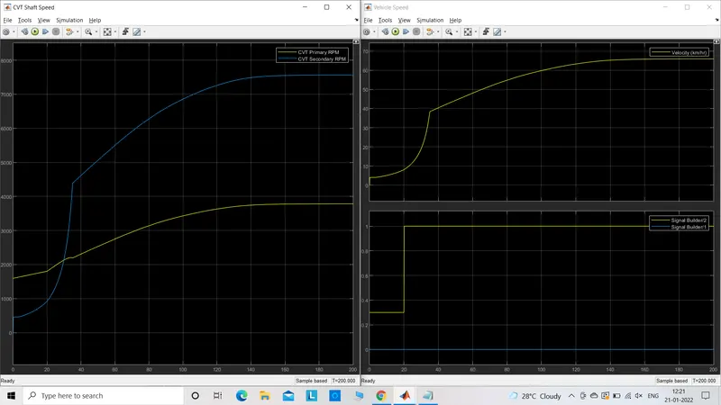
The cvt graph shows that primary pulley rpm rises when the throttle is applied or the vehicle accelerated but the rise is slow and around 1600 rpm. The secondary pulley rpm curve shows a quick rise as it is responsible to increase the speed of the wheels. The rpm which was 500 initially reaches 7500 which means this is set to a high gear and the vehicle is travelling at a fast pace.
The next graph has throttle and brake curve which is 0 for braking and throttle as explained earlier, it remains 0.3 initially but the value reaches to 1 which means throttle is applied to move the car. The other curve is the speed of the car which is quite similar to the secondary pulley rpm curve as they both are connected to each other. The vehicle speed up from 0 to 40 quickly as throttle input is strong and then the speed increase is gradual for the next remaining time till 200 secs. The car reaches 65km/h.
2)Atv model with dashboard
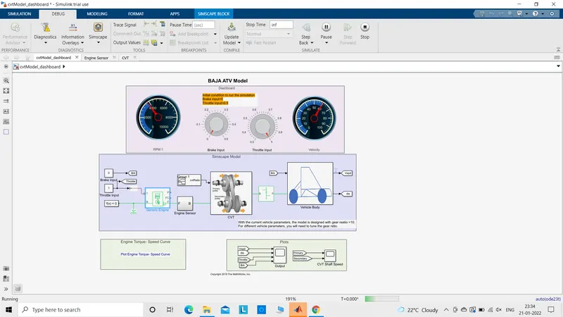
This model is same as model 1 but has an additional dasboard controlls which show the input and output values as mentioned earlier. Whatever changes are sensed by the engine sensor is displayed on the rpm analog meter. Same goes for speedometer where the whatever change in speed is experienced by the vehicle is displayed on the speedometer. So the input are given by the knobs provided for brake and throttle each instead of a signal builder. The motive behind this model is to study the effect of braking and throttle on the vehicle velocity and rpm. Initial throttle is set to 0.5 and brake is set to 0. As I was controlling the knobs in different manner for throttle and brake, I got different output of rpm and velocity of the car. The velocity decreased when brake was set to 0.5 and throttle undisturbed. The car came to a halt when throttle and brake were brought to 0 and there was more rpm into action according to the model. The rpm reached 4000 rpm and velocity reached 60km/h when full throttle was given with 0 brake input.
3)ATV with help of look-up table without dashboard
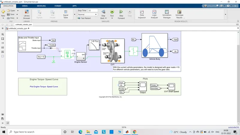
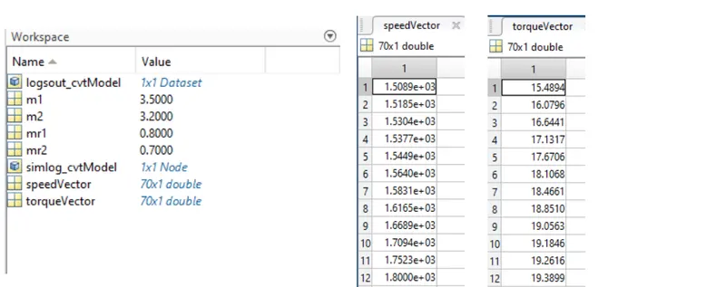
The whole model is the same as model 1 but here instead of signal builder, a lookup table is used as an input to the cvt tranmission. The table was initially loaded in the MATLAB and it was in form of a spreadsheet and is visible in the workspace as mentioned earlier. The engine over here is mapped with a predefined array of values which is loaded. This array is mapped with the output values. This will create a mathematical function. By inputing the values, the look-up table would bring the corresponding output values from the table. The lookup table would create a lookup operation to get the output values and also uses interpolation, extrapolation or rounding method top find the output values in case if it fails to get the values from the corresponding table.
The output graph is:-
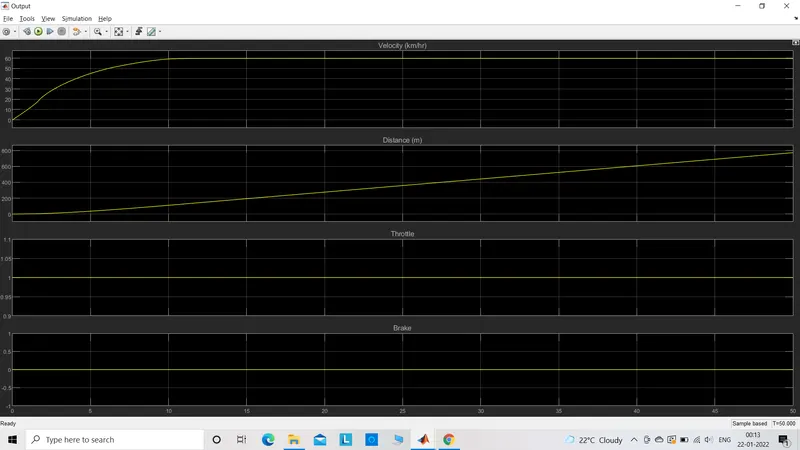
The brake is not applied but throttle is given with a value 1 for entire 50 secs. The vehicle starts moving and the distance covered by it is indicated linearly in the graph. Initially the car begins in a very lazy manner but then the the distance covered in each sec then increased in a constant manner upto 50 secs.
Velocity of the car is observed in the graph shows that for 10 secs the increase in the velocity is pretty impressive but then after 10 secs the velocity becomes constant because the throttle is maintained at input value 1. The initial torque of the car is good according to this model which shows a quick 0-60 km/h in 10 secs for a vehicle which is made for off-road. This shows that the torque applied on the wheel brings the wheels to reach a velocity of 60km/h which would prove to be helpful in harsh off-road conditions.
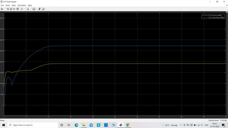
The primary pulley starts around 1700rpm above secondary pulley initially. Because intially torque is required to vring the car in motion and this could be achieved when diameter of the primary push belt is smaller than the diameter of the secondary pulley side push belt. The secondary belt starts moving faster than the primary and it overtakes the primary pulley around 3100 rpm. This is done when the diameter of the push belt rotating on the secondary pulley starts decreasing and there is a increase in the diameter of the primary pulley push belt. This rise is seen until the car reaches 60 km/h which is the best the throttle of 1 could make change in the velocity of the car. This was seen that the car reached 60km/h at 10th sec and here also the curve climbes only till 10 secs and then the rise is not visible. The throttle is set to 1 and so then both the pulleys remain in that same diameters and so the curve becomes a straight horizon indicating no more change uptil 50 secs.
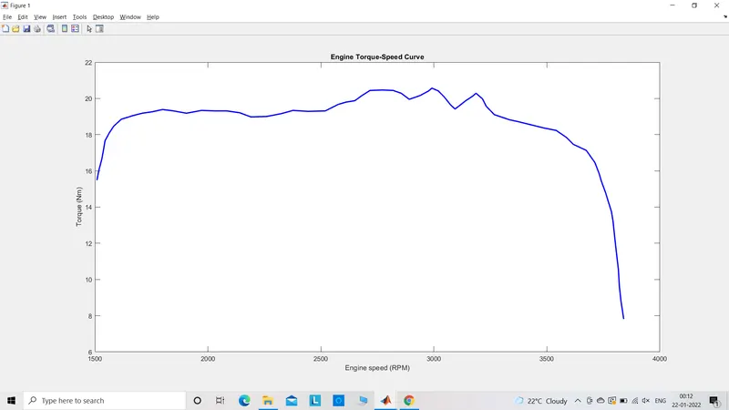
The above graph is between rpm and torque. It shows that initially the throttle is given and so the torque increases and also making the engine to increase the rpm. I assumed that the car was already turned on with initial rpm of 1500 which was produced due to that 15-16Nm of torque as shown in the figure. It increases quickly to reach 19 and then rises and falls gradually but remains inside the torque range 18-20 Nm till 2500rpm. This is according to be is because the throttle is set to a constant value. The curve shows some small fluctuations till 3300 rpm which and this is the region when the car reached its top value of torque 20Nm. The later region experiences a fall in the curve which means there is no more torque getting used to make the engine to run. Very less torque is now used to remain the engine in running condition and the rpm reaches 3800 rpm quicker as comparatively.
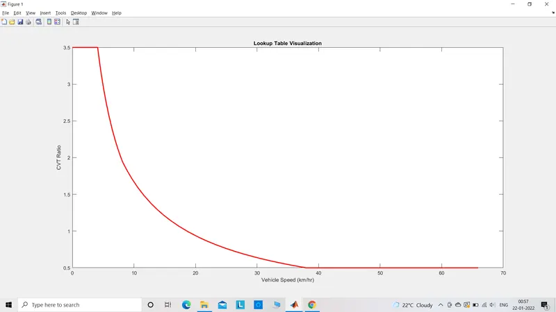
The lookup table states that the gear ratio varies from 3.5 to 0.5 and the ratio decreses as the speed of the vehicle increases. The graph shows that the car reached around 67km/h of speed with top gear ratio of 0.5.
4) Model using look-up table with dashboard
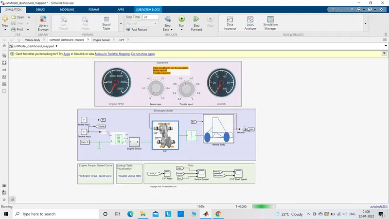
The model is same as model 3 but here we have a dasboard to display the changes in the vehicle. The input is provided with help of look-up table. Look-up table are the synced array of values inputed and then used by the model to give out the output. Here lookup table is provided as an input to cvt transmission.
The increasee in the throttle means that more fuel and air mixture is allowed to enter the cylinder and so the power and torque both independently increases.
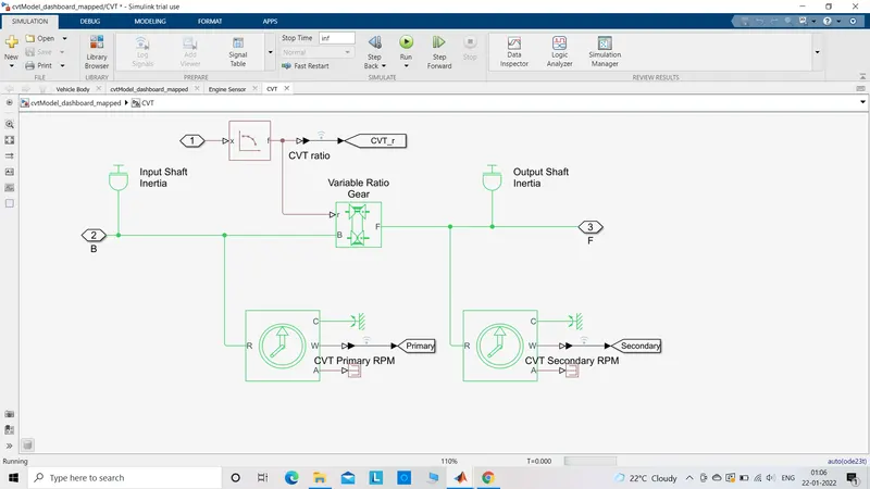
The knobs corresponding brake and throttle is rotated and the following graphs were produced,
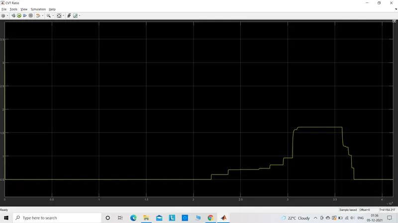
The above graph shows cvt ratio which is at 3.5 initially but comes to 0.5 as the vehicle is provided with great throttle input. It remains at 0.5 for some time means the throttle was set to constant. Then later brake was applied with same throttle input so the increase in the ratio is slow but when the throttle was also reduces then the graph rose which increased the cvt to cross 1.5 ratio. In the end the brake was released and the throttle was again given to improve the gear ratio to 0.5 again resulting in increase in the vehcle speed.
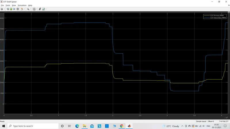
The above graph is between the pulley speeds of both primary and secondary. In the begining the primary pulley was around 1500 rpm. Both the pulleys show an identical variation with primary being at lower rpm for some time which is in between 2000-4000rpm. Secondary was at 0 rpm but rose to 6800rpm and then remained at this mid rpm range but above primary no doubt. This meant that the vehicle is increasing its speed and then showed some variation. The rpm of both pulley drops which means the vehcile is deccelarating now and then the rpm of secondary dropped further and gone below primary which meant that the car was then moving in low gear or high cvt ratio and low speed. The speed again increased and the engine reached at high gear when the throttle was provided. This could be seen in the graph where the secondary pulley rpm crossed primary pulley's rpm and rose further. The highest the secondary pulley reached was 7500 rpm and primary pulley reached 3800 rpm. All the behaviour was in conjuction with the operation of the brake and throttle knobs.
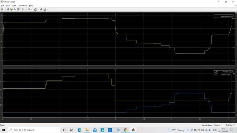
The graph shows the behaviour of vehicle speed with respect to throttle and brake input. When the brake was 0 and the throttle was constant, the car was moving at a constant speed but when the throttle was increased a bit the speed also increased accordingly. Then, the throttle was dropped and slowly the brakes were applied and this affected the car such that the speed reduced gradually. The throttle was brought to it's minimum value of 0.3 and braking action was increased which made the car to further reduce the speed. In the end, the brake was released and the throttle was provided quickly which increased the speed of the car quickly. These models will help the ATV cvt developers to run and simulate the type of gear ratio and the effect of throttle, brake on the performance of the vehcile which would help in developing a better ATV for the challenge.
The report was prepared and all the cases are well recorded and provided systematically.