Project
Objective: To carry out a system-level simulation of an all-terrain vehicle and to make a technical report explaining model properties and discussion on results.
Theory:
All-terrain vehicle (ATV):
An all-terrain vehicle (ATV) is defined as a motorized off-highway vehicle designed to travel on four low-pressure or non-pneumatic tires, having a seat designed to be straddled by the operator and handlebars for steering control.
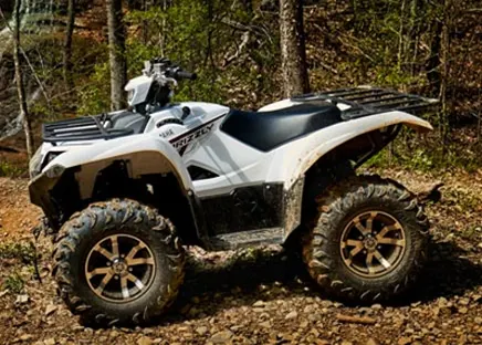
Major components used in simulation:
Signal Builder: Used to provide throttle and brake input.
Generic Engine:
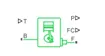
This block represents system-level spark ignition diesel engine, where ports: T is the input for throttle, B and F are mechanical rotational conserving ports, P and FC are output ports of engine power and fuel consumption rate respectively.
RPM sensor:

This block represents an ideal RPM sensor, that converts the input RPM into a control signal in the form of angular velocity and displacement from the A and W port respectively.
CVT transmission: Continuous variable transmission is an automatic type transmission that has a continuous range of gear ratios, through which smooth speed change can be achieved compared to gear ratio in fixed steps. Also with suitable control, the engine rpm can be kept constant under variable speed conditions.
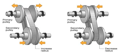
In a typical CVT, there are two shafts on which taper discs are mounted, these two shafts are connected with a belt, When the discs on a particular shaft come closer or depart away from each other, the radius on which the belt mounted changes to achieve seamless change in gear ratio.
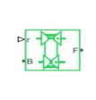
Here R is the input port for the CVT ratio, B and F base and follower pulley ports respectively.
Simple gear:

A gear ratio of a simple gear can be defined as
Gear ratio = Follower gear speed/Base gear speed(Nf/Nb)
This block represents a simple gear where ports B and F are mechanical rotational conserving ports.
Vehicle Body:
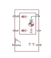
This block represents the vehicle body, which is a representation of two-axle vehicle with longitudinal motion. The vehicle parameters such as body mass, aerodynamics drag, and inclination angle of the road, can be specified.
Port H is a mechanical translational conserving port, V, NF, and NR are output ports for a physical signal for vehicle velocity, front, and rear wheel force respectively. W and beta are input port for headwind speed and road inclination.
Double shoe brake: For braking double shoe brake are used

Where port s is the rotational conserving port associated with the drum shaft and port F is the input port of the physical signal to the actuator.
Tire:

This block represents the tire model used in the simulation, where port A and H is mechanical rotational and translational conserving port respectively. Port N is the physical signal input port that applies the normal force on the tyre, and port S is for output signal for slip
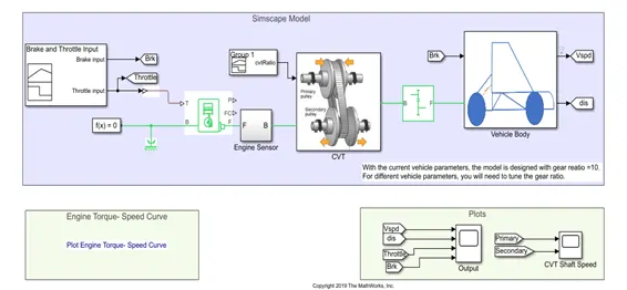
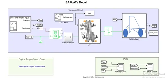
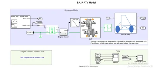
Simulink Model 1: This is the main model, in which throttle, brake, and CVT ratio input is provided from a signal builder block. The simple gear ratio used here is Nf/Nb =10.
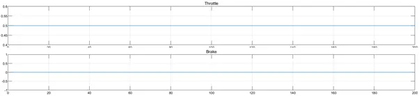
Speed throttle and brake inputs are provided with the help of signal builder block, here throttle is maintained constant at 0.5, and brake input is 0 which can be seen in the plot shown below.
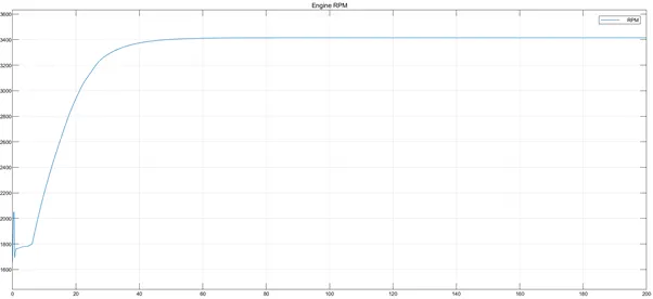
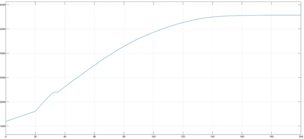
As there is no break input provided engine rpm kept on increasing and after about 40s settles at 3400 rpm, the plot of engine rpm is shown below
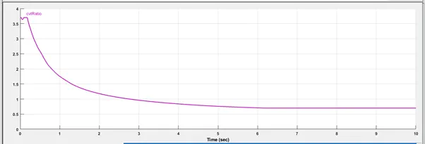
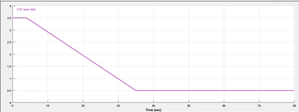
The output speed of the generic engine is fed to a CVT model whose CR ratio in this model is provided by using a signal builder block, CVT ratio is provided is shown below.
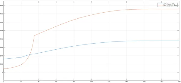
The CVT primary and secondary shaft rpm is shown below
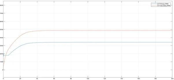
Form the above figure it is clear that when the CVT ratio is greater than 1 the primary shaft speed is more than the secondary shaft speed and vice-versa.
Also the speed of the vehicle and the distance covered by it is shown in the figure below
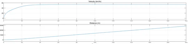 \
\
A simple gear with gear ratio of 10 is used here after the CVT secondary shaft.
The engine toque speed characteristic is shown in the plot below.
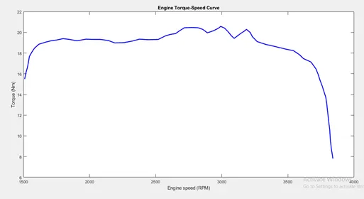
As same specification generic engine used in all model so the engine torque Vs speed curve is same for all models.
Simulink model 2:
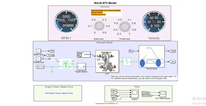
This model includes a dashboard for RPM of the engine and a speedometer for the vehicle velocity. Also the brake and throttle inputs are provided by two nobs. Initially, the brake input is at zero, and the throttle input is at 0.5. Simulation results are shown below.
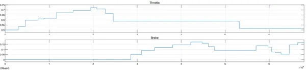
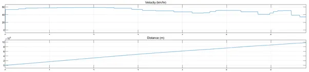
Step change in the throttle and brake input provided is shown above and velocity and distance covered by vehicle is shown below
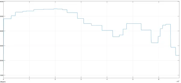
Engine RPM plot is shown below:
The CVT primary and secondary shaft RPM is shown below:
Simulink Model 3: In this model the CVT ratio input is loaded in to work space as ‘cvtr’ which is used in the subsequent models, for formation of the lookup table of CVT ratio input. In further models simple gear ratio Nf/Nb =12 is used.
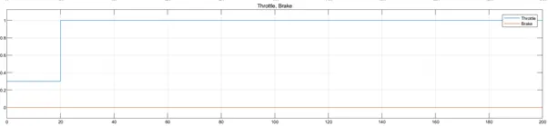
Throttle and brake input plot:
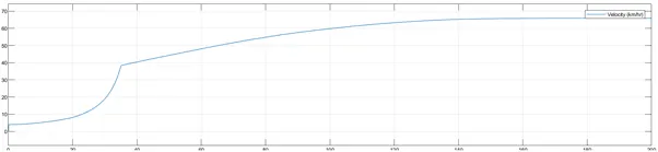
Vehicle speed plot:
CVT ratio input plot:
Engine RPM plot:
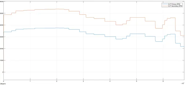
CVT primary and secondary shaft RPM plot:
Simulink model 4: In this model, the CVT gear ratio is provided from a 1-D lookup table by using the CVT ratio or model 3 as table data and speedV as breakpoints.
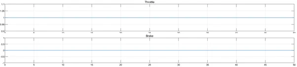
Brake and throttle input plot: Brake and throttle inputs are provided by using signal builder block
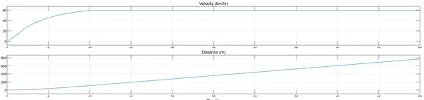
Vehicle velocity plot:
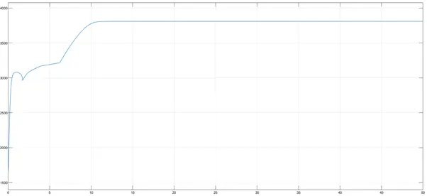
Engine RPM plot:
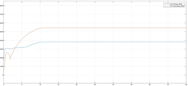
CVT primary and secondary shaft RPM plot:
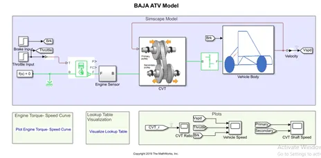
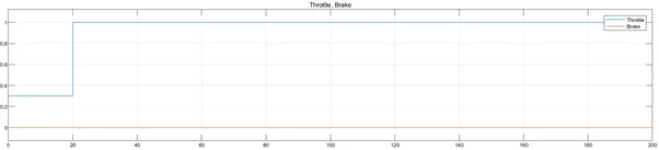
Simulink model 5: In the following models the CVT ratio input is provided from the lookup table formulated from the feedback of the vehicle speed instead of input from a signal builder block. The brake and throttle input provided from signal builder block.
Brake and throttle input plot:
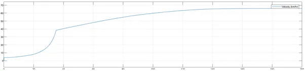
Vehicle velocity plot:
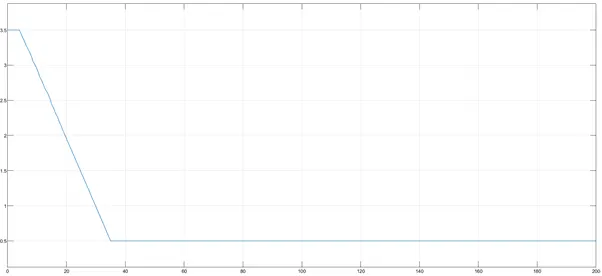
CVT gear ratio input plot:
CVT primary and secondary shaft RPM plot:
Engine RPM plot:
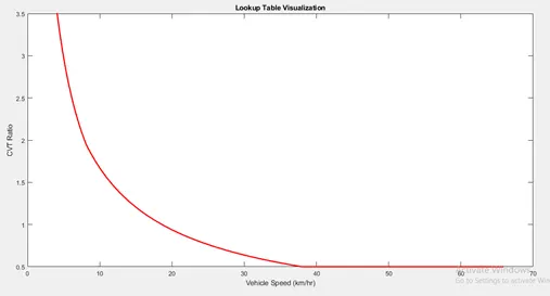
Lookup table visualization: Plot of CVT ratio vs vehicle speed
Simulink Model 6:In this simulation model a dashboard is provided for engine RPM and vehicle velocity
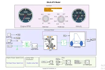
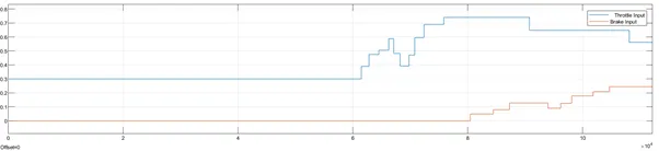
Throttle and Brake inputs are provided by using nobs. Initially, the throttle input nob is set at 0.3 and brake input nob at 0, after that step inputs are provided as shown below:
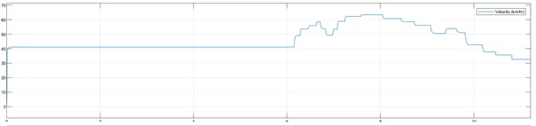
Vehicle velocity plot:
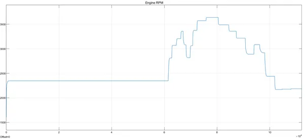
Engine RPM plot:
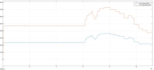
CVT primary and secondary shaft RPM plot:
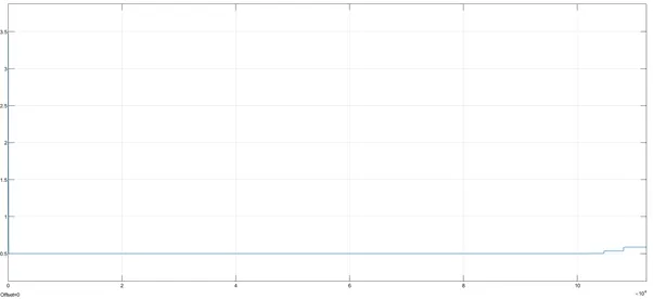
CVT ratio Plot:
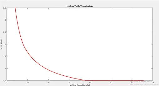
Lookup table visualization: Plot of CVT ratio vs vehicle speed
Conclusion: Simulation of BAJA ATV, with different brake, throttle, and CVT ratio is simulated and their results are obtained successfully.