BAJA ATV
BAJA ALL-TERRAIN VEHICLE (ATV) ANALYSIS
AIM: To study The baja all-terrain vehcile(ATV) model using simulink, to wrtite a technical report on the model parameters and results.
Software Used: MATLAB - SIMULINK ( Version R2021a)
Introduction:
All-Terrain Vehicle:
- An all-terrain vehicle (ATV) is defined as a motorized off-highway vehicle designed to travel on four low-pressure or non-pneumatic tires, having a seat designed to be straddled by the operator and handlebars for steering control.
- It is also known as a quad or quadricycle type vehicle.
- The development of the All Terrain Vehicles started way back in the early 19th century. In 1893, Royal Enfield manufactured and sold the first powered quadricycle. The vehicle employed many bicycle components such as the handle bars. However, it was mainly designed for use as a horseless carriage for road use.
- ATVs are subdivided into two types as designated by the manufacturer
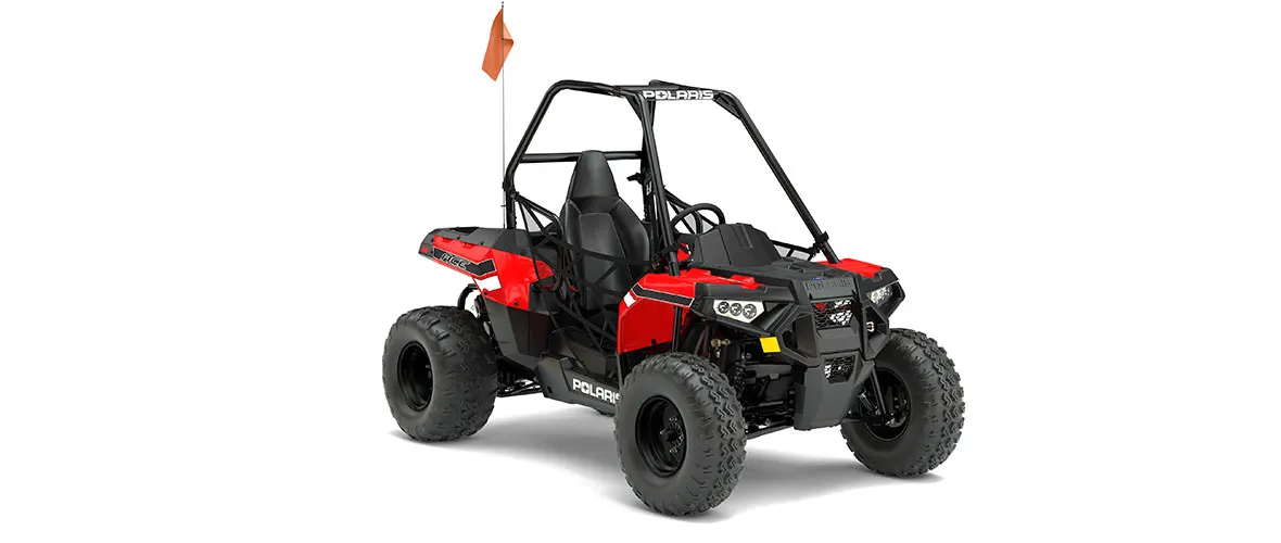
Type I ATVs are intended by the manufacturer for use by a single operator and no passenger.
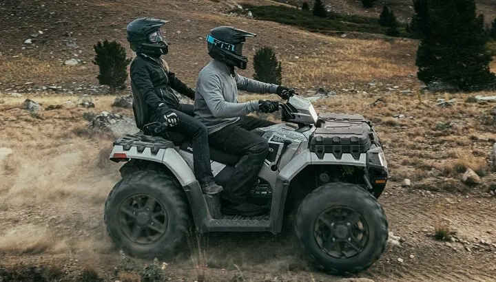
Type II ATVs are intended by the manufacturer for use by an operator and a passenger, and are equipped with a designated seating position behind the operator.
BAJA ATV (SAE):
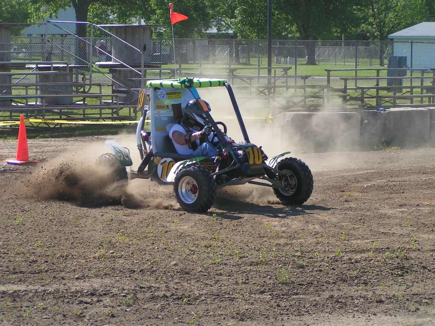
- Baja SAE is an intercollegiate design competition run by the Society of Automotive Engineers (SAE). Teams of students from universities all over the world design and build small off-road cars. The cars all have engines of the same specifications.
- As of 2009 the engine has been an unmodified Briggs & Stratton Intek 20 single-cylinder with a displacement of 300cc and power output of approximately 10 bhp (7.5 kW).
- The goal in Baja SAE racing is to design, build and race off-road vehicles that can withstand the harshest elements of rough terrain. The vehicles used in Baja SAE racing are often similar in appearance to dune buggies.
- There are multiple dynamic events, usually four per event, as well as a single four-hour endurance race. The dynamic events include hill climbs, chain pulls, maneuverability events, rock crawls, and suspension & traction events.
- Static events, such as written reports, presentations and design evaluations are provided by participating teams. This is when the teams are judged on ergonomics, functionality, and producibility of their cars; ensuring that the final placement of the team does not rest solely on the vehicle's performance but rather on a combination of static and dynamic events.
- Required reports detail the engineering and design process that was used in developing each system of the team’s vehicle, supported with sound engineering principles.
- Also, a cost report that provides all the background information necessary to verify the vehicle’s actual cost is used to rate the most economically feasible for production.
- The most rugged of all the competitions, Baja SAE also gives students the first-hand challenge of pursuing their passion while managing real-life demands and priorities.
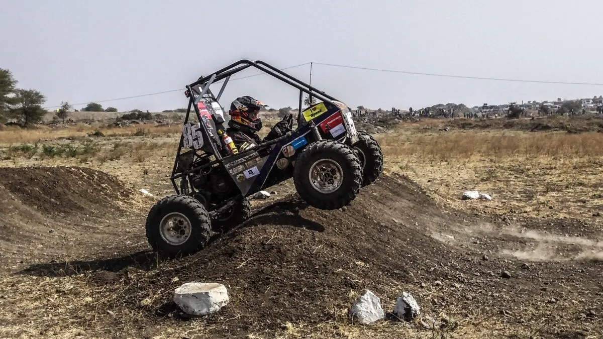
- Each team's goal is to design and build a prototype of an all-weather, rugged, single-seat, off-road recreational vehicle intended for sale to the nonprofessional weekend off-road enthusiast.
Important components of BAJA AVT In Simulink Model:
a) Generic Engine:
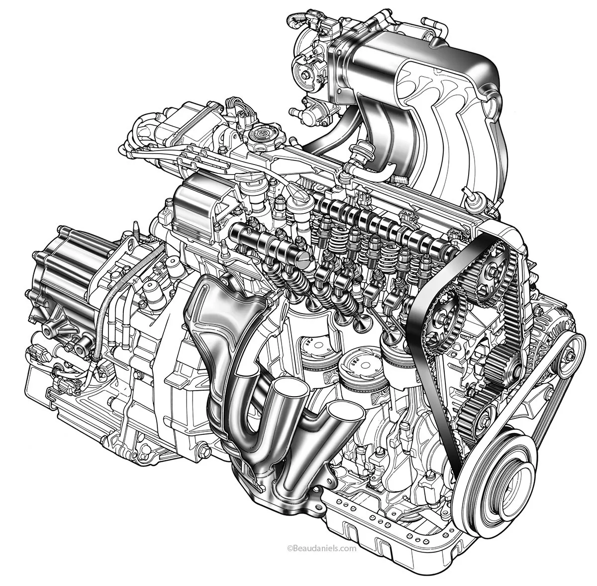
- The Generic Engine block represents a general internal combustion engine which is suitable for spark-ignition and diesel. Speed-power and speed-torque parameterizations are provided.
- A throttle physical signal input specifies the normalized engine torque. Optional dynamic parameters include crankshaft inertia and response time lag.
- A physical signal port outputs the engine fuel consumption rate based on the fuel consumption model that you choose. Optional speed and redline controllers prevent engine stall and enable cruise control.
Engine speed, Throttle, Power and Torque:
- By default, the Generic Engine block uses a programmed relationship between torque and speed that is modulated by the throttle signal.
- The block evaluates engine power demand as a function of engine speed, g(Ω). The function provides the maximum power available for a given engine speed, Ω. The block parameters—Maximum power,Speed at maximum power,and Maximum speed— normalize this function to physical maximum torque and speed values.
- The normalized throttle input signal T specifies the actual engine power. The power is delivered as a fraction of the maximum power possible in a steady state at a fixed engine speed.
Engine Power Demand:
- The engine power is nonzero when the speed is limited to the operating range, Ωmin ≤ Ω ≤ Ωmax. The absolute maximum engine power Pmax defines Ω0 such that Pmax = g(Ω0).
- Define w ≡ Ω/Ω0 and g(Ω) ≡ Pmax·p(w). Then p(1) = 1 and dp(1)/dw = 0. The torque function is:
τ = (Pmax/Ω0)·[p(w)/w].
- You can derive forms for p(w) from engine data and models. The Generic Engine block uses a third-order polynomial form
p(w) = p1·w + p2·w2 – p3·w3
Typical Engine Power Curve:
- The block restricts the engine speed to a positive range above the minimum speed and below the maximum speed: 0 ≤ wmin ≤ w ≤ wmax.
- The engine power at minimum speed must be nonnegative: p(wmin) ≥ 0. If you use the polynomial form, this condition is a restriction on the pi:
- p(wmin) = p1·wmin + p2·w2min – p3·wmin3 ≥ 0.
- The engine power at maximum speed must be nonnegative: p(wmax) ≥ 0. If you use the polynomial form, this condition is a restriction on wmax: wmax ≤ w+.
Engine Power Forms for different Engine Types:
| Power Demand Coefficient |
Spark Ignition | Diesel |
| p1 | 1 | 0.6526 |
| p2 | 1 | 1.6948 |
| p3 | 1 | 1.3474 |
Idle Speed Controller Model:
- The idle speed controller adjusts the throttle signal to increase engine rotation below a reference speed according to the following expressions:
d(Πc)/dt=0.5⋅(1−tanh(4⋅ω−(ωr/ωt)))−Πc/τ where: Π is the engine throttle, Πi is the input throttle (port T), Πc is the controller throttle, ω is the engine speed or crankshaft angular velocity, ωr is the idle speed reference, ωt is the controller speed threshold, τ is the controller time constant.
- The controlled throttle increases with a first-order lag from zero to one when engine speed falls below the reference speed.
- When the engine speed rises above the reference speed, the controlled throttle decreases from one to zero.
- When the difference between engine velocity and reference speed is smaller than the controller speed threshold, the tanh part of the equation smooths the time derivative of the controlled throttle.
Redline Controller Model:
- While the idle speed controller determines the minimum throttle value for maintaining engine speed, the redline controller prevents excessive speed based on a maximum throttle input.
- To determine the maximum throttle value, the redline controller uses the idle speed controller model equation. However, for the redline controller:
ωr is the redline speed reference, ωt is the redline speed threshold, τ is the redline time constant.
Performance:
- To increase simulation speed, set Fuel consumption model to
No fuel consumption. - The block solves the equation even if the FC port, which reports the fuel consumption rate, is not connected to another block.
- When the parameter is set to
No fuel consumption, the block does not calculate fuel consumption, even if the FC port is connected to another block.
Assumptions and Limitations:
-
This block contains an engine time lag limitation.Engines lag in their response to changing speed and throttle. The block optionally supports lag due to a changing throttle only. Time lag simulation increases model fidelity but reduces simulation performance.
Ports:
Input:
T — Normalized engine throttle level, unitless, physical signal. Engine torque demand as a fraction of maximum possible torque.
Output:
P — Instantaneous engine power, W, physical signal. Power produced by the engine, in W.
FC — Fuel consumption rate, kg/s, physical signal. Fuel consumed by the engine, in kg/s.
Conserving:
B — Engine block, mechanical rotational. Mechanical rotational conserving port associated with the engine block. This is the base port. The engine block is the physical body that contains the piston cylinders.
F — Engine crankshaft, mechanical rotational. Mechanical rotational conserving port associated with the engine crankshaft. This is the follower port of engine. The crankshaft transmits the power generated from the combustion process. Typically, you attach a clutch and transmission at this port.
b) CVT:
- The CVT Controller block implements a push belt continuously variable transmission (CVT) controller. The block uses standard pulley and geometric equations to calculate the kinematic setpoints for the CVT variator.
- A CVT, or continuously variable transmission, seamlessly changes through an unending range of effective gear ratios while you drive, whereas other kinds of mechanical transmissions offer a fixed number of gear ratios and have hard shifts between each as explained by Certified Transmission Repair. CVT transmission systems are also known as single-speed, shiftless, and stepless transmissions.
- The shiftless nature of a CVT offers unparalleled flexibility that maintains constant angular velocity regardless of output speed. Additionally, a continuously variable transmission makes accelerating smooth and offers enhanced fuel economy.
- The Variable Ratio Transmission block represents a gearbox that dynamically transfers motion and torque between the two connected driveshaft axes, base and follower.
- While a traditional transmission uses a wide variety of intricate parts to shift between a range of preset gears, most CVT systems work through a pulley system. In short, this system consists of cones at each pulley connected via a chain belt. The cones can move to increase or decrease the belt diameter to change gear ratios, allow for quick shifting into the needed ratio for increased power, and boost fuel economy.
- One pulley in the CVT is connected to the engine and the other directs power to the wheels. The width of these pulleys changes based on the needed power; as one gets larger, the other gets smaller. This allows a CVT to deliver strong.
- There is a second, less common, type of CVT that uses a series of discs and rollers, but it operates on similar principles.
- Though there are no gears in a CVT, some simulate a more traditional changing of gears. In these transmissions, the belt-and-pulley system is designed to move to preset points by using a traditional shift lever or paddle shifters on the steering wheel.
- Ignoring the dynamics of transmission compliance, the driveshafts are constrained to corotate with a variable gear ratio that you control. You can choose whether the follower axis rotates in the same or opposite direction as the base axis. If they rotate in the same direction, ωF and ωB have the same sign. If they rotate in opposite directions, ωF and ωB have opposite signs.
- Transmission compliance introduces internal time delay between the axis motions. Therefore, unlike a gear, a variable ratio transmission does not act as a kinematic constraint. You can also control torque loss caused by transmission and viscous losses.
Ideal Motion and Torque Transfer:
- Variable Ratio Transmission is a dynamical mechanism for transferring motion and torque between base and follower.If the relative compliance ϕ between the axes is absent, the block is equivalent to a gear with a variable ratio gFB(t).
Assumptions:
- You can estimate the base angular compliance kp from the transmission time constant tc and inertia J.
- You can estimate the base angular velocity compliance kv from the transmission time constant tc, inertia J, and damping coefficient C.
Nonideal Torque Transfer and Losses:
- With nonideal torque transfer, τloss ≠ 0. Losses in the Variable Ratio Transmission are modeled similarly to how losses are modeled in nonideal gears.
- In a nonideal gearbox, the angular velocity and compliance dynamics are unchanged. The transferred torque and power are reduced by:
- Coulomb friction (for example, between belt and wheel, or internal belt losses due to stretching) characterized by an efficiency η.
- Viscous coupling of driveshafts with bearings, parametrized by viscous friction coefficients μ.
c) Simple Gear:
-
The Simple Gear block represents a gearbox that constrains the connected driveline axes of the base gear, B, and the follower gear, F, to corotate with a fixed ratio that you specify. You choose whether the follower axis rotates in the same or opposite direction as the base axis. If they rotate in the same direction, the angular velocity of the follower, ωF, and the angular velocity of the base, ωB, have the same sign. If they rotate in opposite directions, ωF and ωB have opposite signs.
Assumptions: - Gear inertia is assumed to be negligible.
- Gears are treated as rigid components.
- Coulomb friction slows down simulation.
Ports:
B — Base, rotational mechanical. Rotational mechanical conserving port associated with the base, or input, shaft.
F — Follower, rotational mechanical. Rotational mechanical conserving port associated with the follower, or output, shaft.
d) Vehcile body:
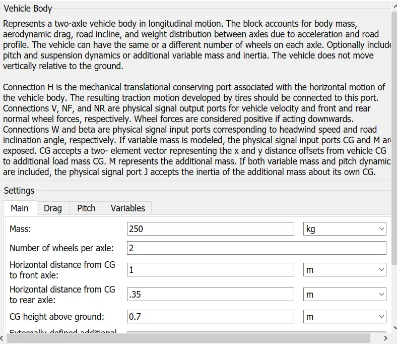
- The Vehicle Body block represents a two-axle vehicle body in longitudinal motion. The vehicle can have the same or a different number of wheels on each axle.
- The block accounts for body mass, aerodynamic drag, road incline, and weight distribution between axles due to acceleration and road profile. Optionally include pitch and suspension dynamics. The vehicle does not move vertically relative to the ground.
- The block has an option to include an externally-defined mass and an externally-defined inertia. The mass, inertia, and center of gravity of the vehicle body can vary over the course of simulation in response to system changes.
Model:
- The vehicle axles are parallel and form a plane. The longitudinal, x, direction lies in this plane and perpendicular to the axles. If the vehicle is traveling on an incline slope, β, the normal, z, direction is not parallel to gravity but is always perpendicular to the axle-longitudinal plane.
| g | Gravitational acceleration |
| β | Incline angle |
| m | Mass of the vehicle |
| h | Height of vehicle center of gravity (CG) above the ground |
| a, b | Distance of front and rear axles, respectively, from the normal projection point of vehicle CG onto the common axle plane |
| Vx | Velocity of the vehicle. When Vx > 0, the vehicle moves forward. When Vx < 0, the vehicle moves backward. |
| Vw | Wind speed. When Vw > 0, the wind is headwind. When Vw < 0, the wind is tailwind. |
| n | Number of wheels on each axle |
| Fxf, Fxr | Longitudinal forces on each wheel at the front and rear ground contact points, respectively |
| Fzf, Fzr | Normal load forces on each wheel at the front and rear ground contact points, respectively |
| A | Effective frontal vehicle cross-sectional area |
| Cd | Aerodynamic drag coefficient |
| ρ | Mass density of air |
| Fd | Aerodynamic drag force |
Limitations and Assumptions:
- The Vehicle Body block lets you model only longitudinal dynamics, parallel to the ground and oriented along the direction of motion. The vehicle is assumed to be in pitch and normal equilibrium.
- The block does not model pitch or vertical movement. As such, the equations assume that the wheels never lose contact. This constraint can result in negative normal forces.
Ports:
Input:
W — Headwind speed, m/s, scalar. Physical signal input port for headwind speed.
beta — Road incline angle, rad, scalar. Physical signal input port for road incline angle.
CG — Center of gravity, m, two-element vector. Physical signal input port for the center of gravity, in m, of the externally-defined mass relative to the CG of the vehicle body.
M — Mass, kg, scalar. Physical signal input port for the mass, in kg, of the externally-defined mass.
J — External moment of inertia, kg*m^2, scalar. Physical signal input port for the moment of inertia, in kg*m^2, of the externally-defined mass.
Note:
- Port CG and M are visible only when the Externally-defined additional mass parameter in the Main settings is set to
On. - Port J is visible only when the Externally-defined additional mass parameter in the Main settings and the Pitch dynamics parameter in the Pitch settings are both set to
On.
Output:
V — Longitudinal velocity, m/s, scalar. Physical signal output port for vehicle longitudinal velocity.
NF — Front axle normal force, N, scalar. Physical signal output port for normal force on the front axle. Wheel forces are considered positive if acting downwards.
NR — Rear axle normal force, N, scalar. Physical signal output port for normal force on the rear axle. Wheel forces are considered positive if acting downwards.
Conserving:
H — Horizontal motion, mechanical translational. Conserving port associated with the horizontal motion of the vehicle body. Connect tire traction motion to this port.
e) Tire:
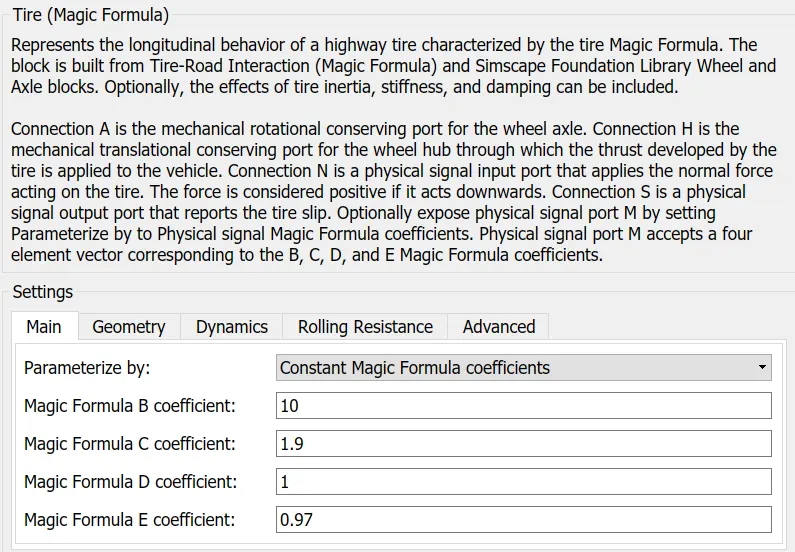
- The Tire (Magic Formula) block models a tire with longitudinal behavior given by the Magic Formula [1], an empirical equation based on four fitting coefficients. The block can model tire dynamics under constant or variable pavement conditions.
- The longitudinal direction of the tire is the same as its direction of motion as it rolls on pavement. This block is a structural component based on the Tire-Road Interaction block.
- To increase the fidelity of the tire model, you can specify properties such as tire compliance, inertia, and rolling resistance. However, these properties increase the complexity of the tire model and can slow down simulation.
Model:
- The Tire (Magic Formula) block models the tire as a rigid wheel-tire combination in contact with the road and subject to slip.
- When torque is applied to the wheel axle, the tire pushes on the ground and transfers the resulting reaction as a force back on the wheel. This action pushes the wheel forward or backward. If you include the optional tire compliance, the tire also flexibly deforms under load.
Dynamics:
- The full tire model is equivalent to this Simscape™/Simscape Driveline™ component diagram. It simulates both transient and steady-state behavior and correctly represents starting from, and coming to, a stop.
- The Translational Spring and Translational Damper are equivalent to the tire stiffness CFx and damping bFx. The Tire-Road Interaction (Magic Formula) block models the longitudinal force Fx on the tire as a function of Fz and k′ using the Magic Formula, with k′ as the independent slip variable.
- The Wheel and Axle radius is the wheel radius rw. The Mass value is the effective mass, Iwr2w. The tire characteristic function f(k′, Fz) determines the longitudinal force Fx. Together with the driveshaft torque applied to the wheel axis, Fx determines the wheel angular motion and longitudinal motion.
- Without tire compliance, the Translational Spring and Translational Damper are omitted, and contact variables revert to wheel variables. In this case, the tire effectively has infinite stiffness, and port P of Wheel and Axle connects directly to port T of Tire-Road Interaction (Magic Formula). Without tire inertia, the Mass is omitted.
Assumptions and Limitations
- The Tire (Magic Formula) block assumes longitudinal motion only and includes no camber, turning, or lateral motion.
- Tire compliance implies a time lag in the tire response to the forces on it. Time lag simulation increases model fidelity but reduces simulation performance.
Ports:
Input:
N — Normal force, physical signal. Physical signal input port associated with the normal force acting on the tire. The normal force is positive if it acts downward on the tire, pressing it against the pavement.
M— Magic formula coefficients, physical signal | vector. Physical signal input port associated with the Magic Formula coefficients. Provide the Magic Formula coefficients as a four-element vector, specified in the order
Output:
S — Slip, physical signal. Physical signal output port associated with the relative slip between the tire and road.
Conserving:
A — Axle, mechanical rotational. Mechanical rotational port associated with the axle that the tire sits on.
H — Hub, mechanical translational. Mechanical translational port associated with the wheel hub that transmits the thrust generated by the tire to the remainder of the vehicle.
Note:
- Port M is exposed only if the Main > Parameterize by parameter is set to
Physical signal Magic Formula coefficients.
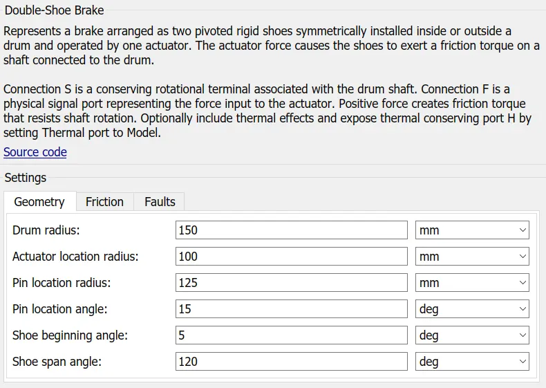
f) Double shoe-brake:
- The Double-Shoe Brake block represents a frictional brake with two pivoted rigid shoes that press against a rotating drum to produce a braking action.
- The rigid shoes sit inside or outside the rotating drum in a diametrically opposed configuration.
- A positive actuating force causes the rigid shoes to press against the rotating drum. Viscous and contact friction between the drum and the rigid shoe surfaces cause the rotating drum to decelerate.
- Double-shoe brakes provide high braking torque with small actuator deflections in applications that include motor vehicles and some heavy machinery.
- The model employs a simple parameterization with readily accessible brake geometry and friction parameters.
Faulty Behavior: When faults are enabled, a belt force is applied in response to one or both of these triggers:
- Simulation time — Faulting occurs at a specified time.
- Simulation behavior — Faulting occurs in response to an external trigger. This exposes port T.
- If a fault trigger occurs, the input force is replaced by the Belt force when faulted value for the remainder of the simulation. A value of
0implies that no braking will occur. A relatively large value implies that the brake is stuck. - You can set the block to issue a fault report as a warning or error message in the Simulink Diagnostic Viewer with the Reporting when fault occurs parameter.
Limitations and Assumptions
- Contact angles smaller than 45° produce less accurate results.
- The brake uses the long-shoe approximation.
- The brake geometry does not self-lock.
- The model does not account for actuator flow consumption.
Ports:
Input:
F — Actuating force, physical signal. Physical signal input port associated with the applied actuating force.
T — External fault trigger, physical signal. Physical signal port for an external fault trigger. Triggering occurs when the value is greater than 0.5. There is no unit associated with the trigger value.
Conserving:
S — Drum shaft rotation, rotational mechanical. Rotational conserving port associated with the rotating drum shaft.
H — Heat flow, thermal. Thermal conserving port associated with heat flow.
Note:
- Port T is visible when Enable faults is set to
Onand Enable external fault trigger is set toOn. - Port H is visible only when, in the Friction settings, the Thermal Port parameter is set to
Model.
Blocks Used:
- Signal Builder - for input of Throttle, Brake and CVT Ratio.
- Generic Engine - Input as Torque and Speed to run the Engine.
- Inertia - To specify the inertia of the vehicle.
- Variable Gear Ratio - To vary the speed according to the gear ratio.
- Double Shoe-brake - to apply the brakes for the vehicle.
- Tire - Rotation and displacement of vehcile.
- Vehicle Body - represents the BAJA ATV vehicle body model.
- Measure Guage - To measure the brake and throttle input.
- Knob - to vary the Throttle and brake inputs.
- Lookup table - For accepting the values from the workspace.
- Simple Gear - reducing the speed by varying the gear ratio.
- Step - increase or decrease input value for specific time interval.
- Rotational Free end - it's a mechanical rotational component.
- PS Terminator - terminate the unconnected physical signal outputs.
- PS Constant - for generating constant physical signal.
- Solver Configuration - for solving the parameters at the start of the simulation.
- Rotational Motion Sensor - to sense the rotation of the mechanical system and give the output.
- Simulink to PS Converter - To convert Simulink signal to Simscape(Physical signal).
- PS Converter to Simulink - To convert Simscape(Physical signal) to Simulink.
- Mechanical Reference - Ground reference to clear any faulty condition while Simulation.
- Scope - To view the plots of the different parameters.
- Display - To display the output value during the Simulation and final value can be viewed at the end of the Simulation.
Model Configuration Types:
- BAJA ATV model without Dashboard.
- BAJA ATV model with Dashboard.
- BAJA ATV model - Mapped Lookup Table without Dashboard.
- BAJA ATV model - Mapped Lookup Table with Dashboard.
BAJA ATV MODEL WITHOUT DASHBOARD:
Main Model:
Engine Sensor:
CVT:
Vehicle Body:
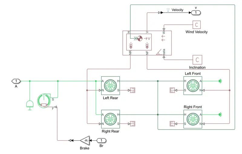
Procedure of Simulation:
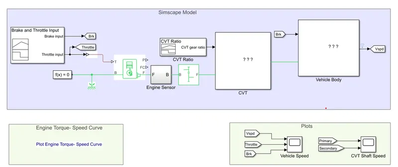
- The Throttle and Brake inputs are generated in the signal builder block.
- The Throttle is then connected to the Engine and Brake is connected as input the vehicle axle.
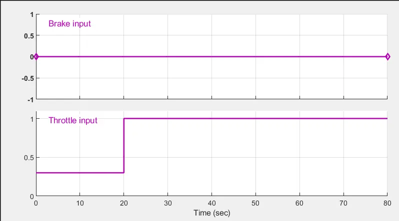
- The brake input is kept as zero i.e., no brake is applied, while Throttle input is apllied as 0.3 for the first 20sec and then increased to 1 for next 20 to 80sec.
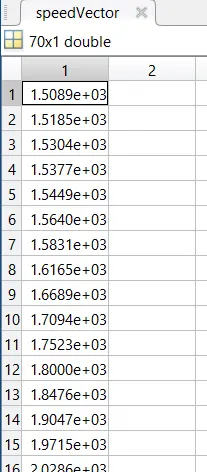
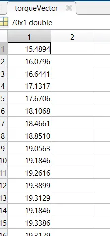
- The speed and torque vectors are predefined in Workspace according to the Torque speed characteristics of the vehicle and these are extracted through grabit in MATLAB.
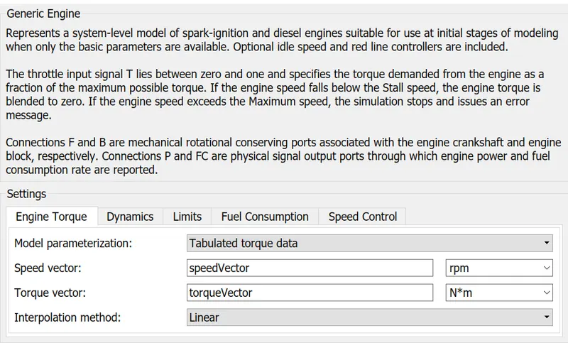
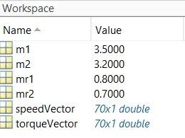
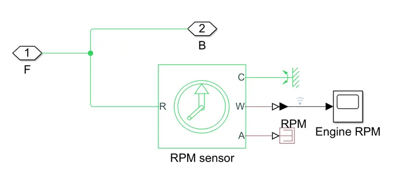
- The output from the Engine is taken from crankshaft and connected to Ideal rotational Sensor to sense the output run from the engine.
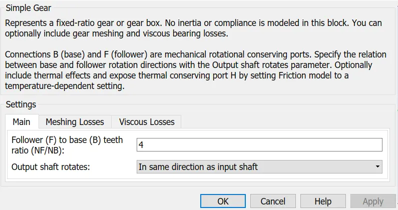
- The Output of the Engine rpm is given to the simple gear mechanism to reduce the speed where the gear ratio is 4.
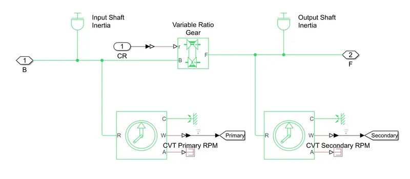
- The output of the gear is given as CVT where the output speed gets reduced.
- The input to Variable Ratio Transmission (CVT block) is provided by Signal Builder.
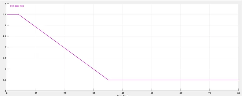
- The output CVT is given as input to the axle by which vehicle accelerates according to the speed, the brake signal generated by signal builder is inputed to the Double shoe-brake of vehicle body to apply the brake to axle.
- The output of the vehicle body is taken as velocity output of the vehicle.
Results:
Torque-Speed Plot:
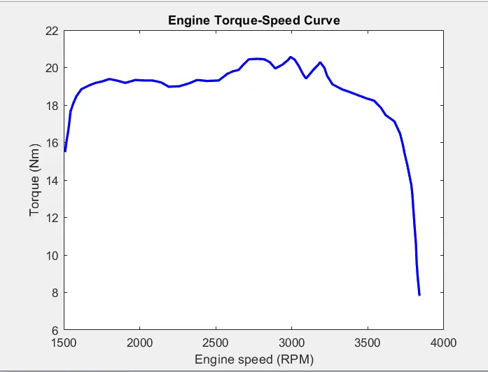
- The Torque, speed values are taken from MATLAB workspace to the engine block to generate the required output rpm. This plot is taken as default input to the engine for all the cases.
Engine speed curve:
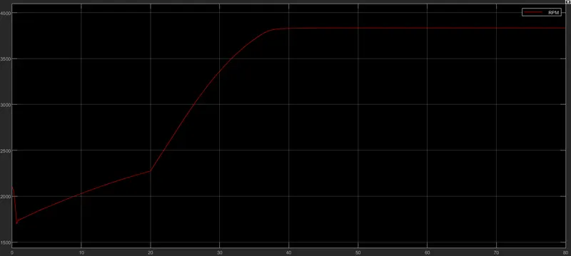
- The output of engine is generated according to the Throttle torque-speed input curve.
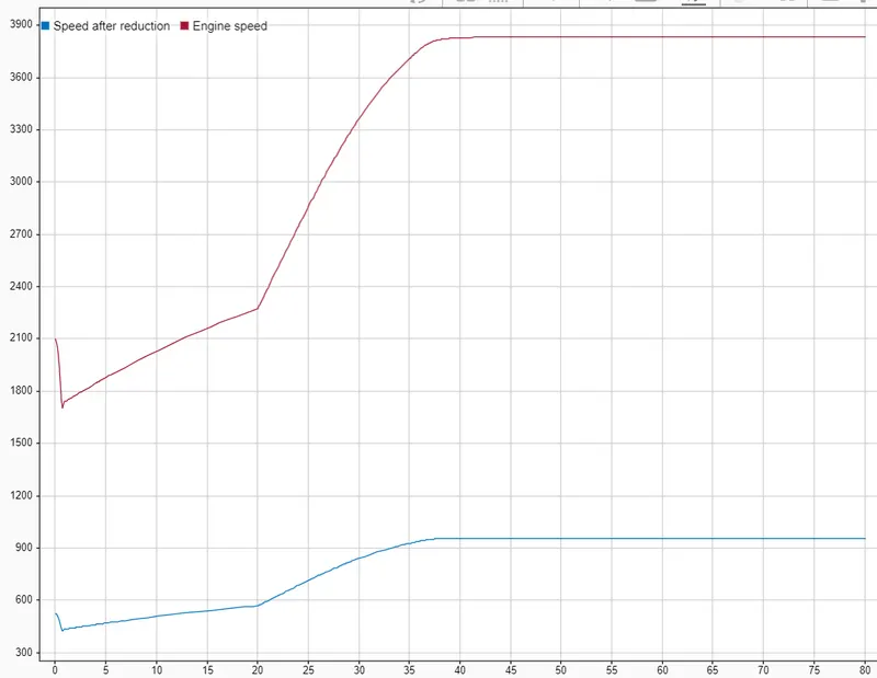
- The engine speed is reduced by the gear ratio '4'.
Max rpm [before reduction] = 3830 rpm.
gear ratio = 1:4
Gear ratio = Driven/Drive
Driven = Drive*gear ratio
Driven = 3832*(1/4)
Driven = 958 rpm
The reduced rpm is 958 which is same as in the plot.
CVT Shaft Reduction Plot:
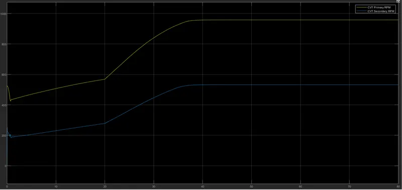
Max Speed [before CVT] = 958rpm
CVT ratio = 1:1.8
Driven = (958/1.8)
Driven = 532.22 rpm
- The reduced max speed after the CVT ratio is 532.22rpm as seen in the plot.
Vehicle speed and Inputs of throttle and brake plot:
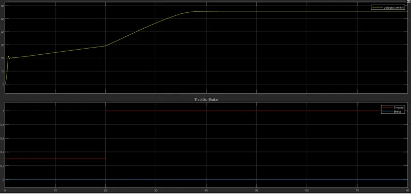
- The input of the throttle is applied as 0.3 for 0-20seconds and then increased as step to 1 from 20-80sec whicle increases the speed of the vehicle.
- The input to the brake is taken as zero throughout the curve.
- From the final vehicle velocity graph we can see that initially there is step rise that is vehicle accelerated faster, then gradually increases for 20sec and then when throtlle increases from 0.3 to 1 the speed also increases i.e accelerates finally reaches the speed and continies to travel at constant speed throughout i.e 55.74kmph.
BAJA ATV MODEL WITH DASHBOARD:
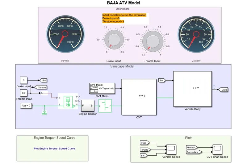
Main model:
Dashboard:
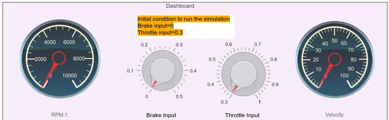
- The model working is similar to that of 'BAJA ATV without dashboard' model but differnce is that their input of throttle and brake is pre-defined but here we can change in the real time while simulation.
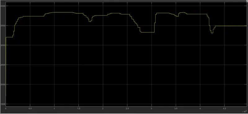
- The engine reduced according to the gear ratio 1:4
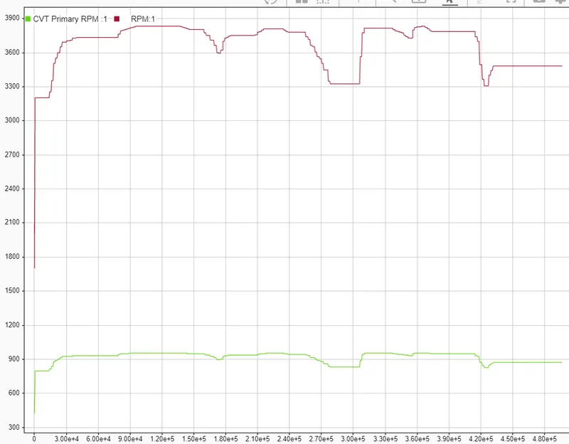
Driven = 3492*0.25
Driven = 873 rpm
- The reduced rpm by the gear is 873rpm.
CVT Shaft Plot:
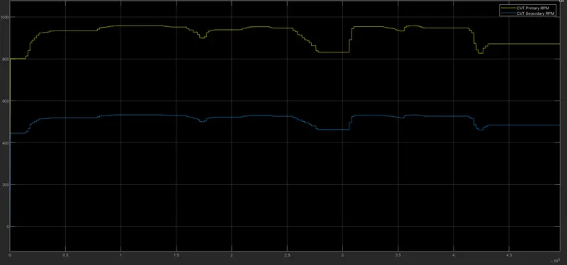
Rpm before CVT = 873 rpm
CVT ratio = 1:1.8
Driven = 873/1.8
Driven = 485 rpm
- The reduced rpm of the CVT output is 485rpm.
Speed and inputs of Throttle and brake plots:
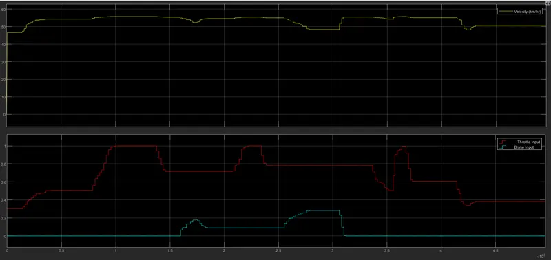
- The input variations of the Throtlle and brake are plotted as throtlle is increased vehicle speed increases and if brake is increases vehicle speed reduces.
- From the final speed plot of vehcile we can see that the initial aceelration of the vehicle is 46kmph average acceleration of the vehicle is 50kmph.
Lookup Table Data Extraction:
Model:
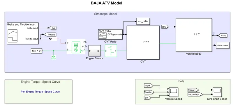
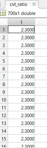
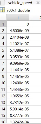
- The model working is same as 'BAJA ATV model without dashborad'. The change is that CVT Ratio and vehicle speed is extrcated from the workspace block.
Worksapce before Data extraction:
Worksapce after Data extraction: 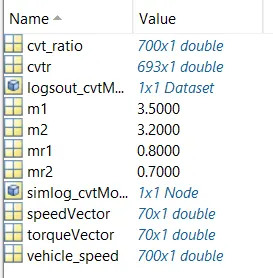
MAPPED LOOKUP TABLE WITHOUT DASHBOARD:
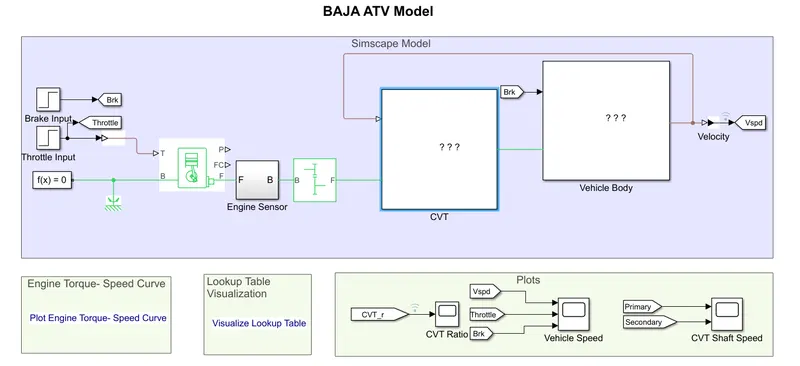
Main Model:
CVT:
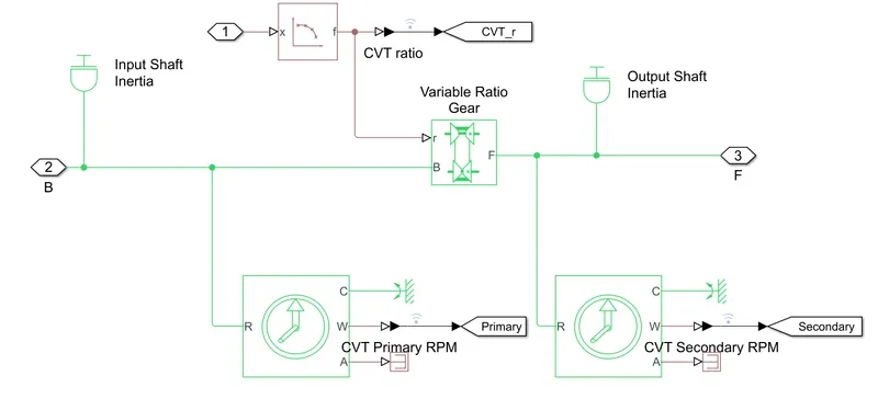
- The working is similar to that of 'BAJA ATV without dashboard model' differnce is that instead of the signal builder block we use step blocks for input of Throttle and brake, 2-D Lookup table for CVT ratio and also feedback of velocity of vehicle back to 2-D lookup table.
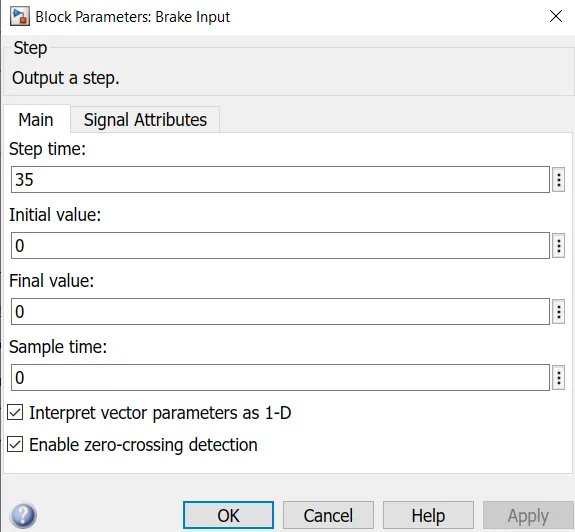
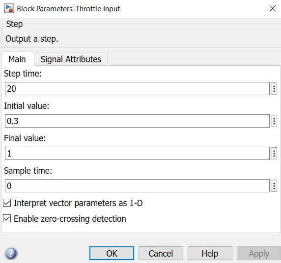
- The brake is input will take value of 0 at time 35sec.
- The throtlle will start with 0.3 as initial value and increases to 1 after 20 sec.
- Instead of CVT singnal builder we have CVT ratio 2-D lookup table.
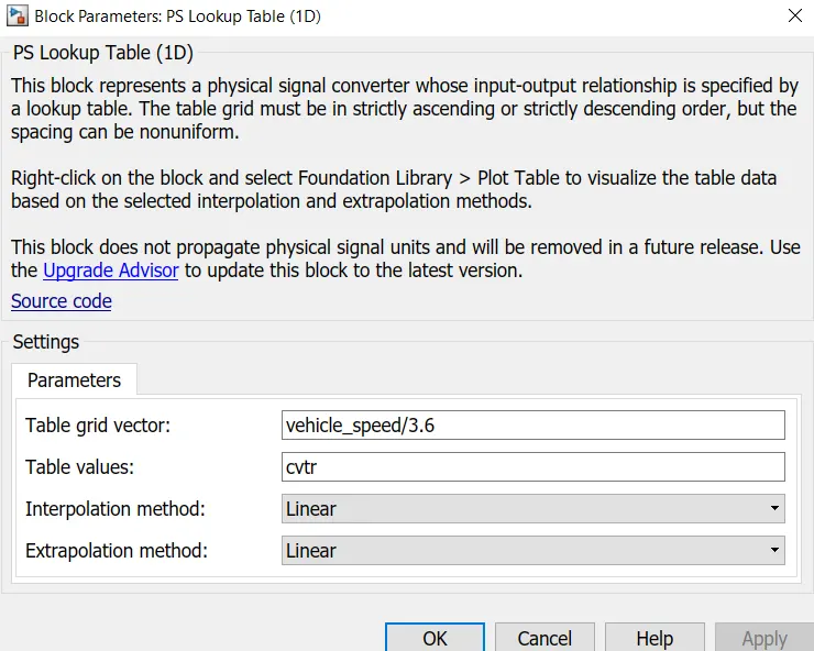
- The vehicle speed is given as feedback to the 2-D lookup table to verify that velocity of vehicle is changing accordingly to the CVT ratio.
Results:
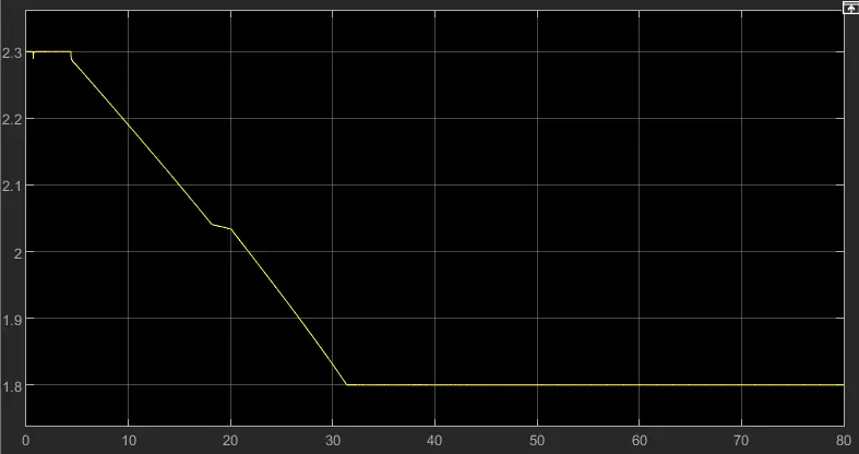
CVT ratio:
CVT ratio and Vehicle velocity:
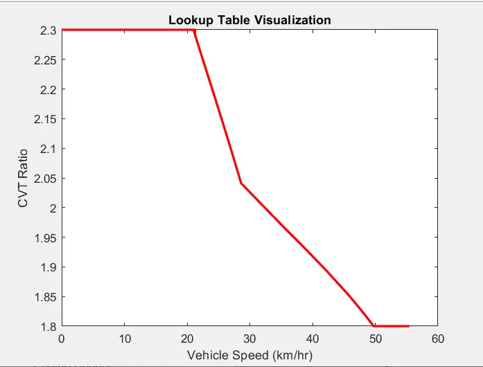
- From plot we can view that CVT varies from 2.3 - 1.8 in 80sec which is similar to 'BAJA ATV without dashboard model'
- The vehcile after 80sec attains a speed of 55.44m/s.
MAPPED LOOKUP TABLE WITHOUT DASHBOARD:
Main Model:
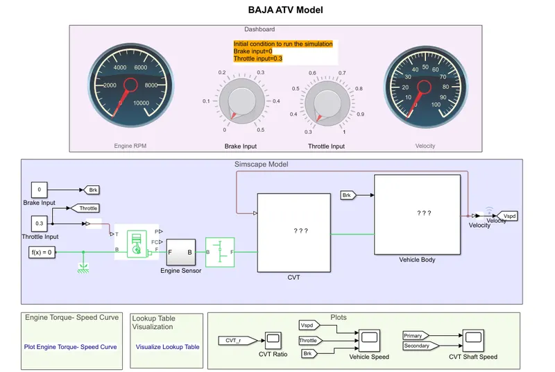
- The process of this model is similar to that of 'BAJA ATV - mapped lookup table without dashborad model' but difference is the throttle and brake input are controlled in real time simulation and feedback to the CVT ratio lookup table.
CVT, Throttle and Brake inputs:
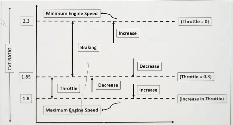
- In this the engine is pre-set to run at 3300rpm for 0.3 throttle value at velocity of 45kmph.
- The CVT ratio for minimum speed is 2.3 and for maximum speed its 1.8 already pre-defined.
- For the starting condition throttle is 0.3 and CVT is 1.88.
- When the throttle is increased the CVT moves towards 1.8 since where it attains maximum speed, adnd when brake is aincreased the CVT moves towards 2.3 which gives the minimum speed.
CVT Ratio plot:
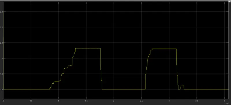
Engine Plot:
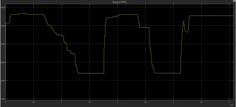
- Drom the graph we can say that vehicle intially running with minrpm 0f 3600 and then after increasing the throttle and braking inputs the engine will be finally settled at 3774rpm as per the inputs.
CVT Speed plot:
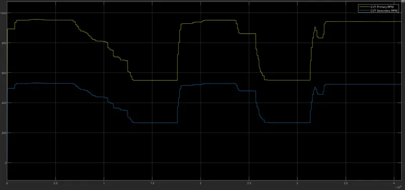
Input and vehicle speed plot:
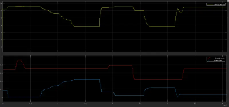
- Hence the vehicle input of the throttle and brake have been plot according to the variation of the input knobs.
- The output velocity is followed according to the inputs of the CVT ratio, Input of throttle and brakes finally running at a constant speed of 54.72kmph.
Conclusion:
Hence a detail technical report of the BAJA ATV by explaining all properties and their results.
References:
- https://www.mathworks.com/matlabcentral/fileexchange/70576-baja-all-terrain-vehicle-atv-model
- Tire with longitudinal behavior given by Magic Formula coefficients - MATLAB - MathWorks India
- Frictional brake with two pivoted shoes diametrically positioned about a rotating drum with triggered faulting - MATLAB - MathWorks India
- Two-axle vehicle with longitudinal dynamics and motion and adjustable mass, geometry, and drag properties - MATLAB - MathWorks India
- Internal combustion engine with throttle and rotational inertia and time lag - MATLAB - MathWorks India