Project_System-level simulation of an BAJA ATV Model-terrain vehicle
1. AIM : Carry out a system-level simulation of an BAJA ATV Model-terrain vehicle.
2. OBJECTIVES OF THE PROJECT:
-
Download the model from here & Prepare a technical report explaining the model properties & comments on the results.
- Perform a simple " BAJA ATV Model " without a Lookup Table.
3.BODY OF THE CONTENT:
`|><|` BRIEF INTRODUCTION :
An All-Terrain Vehicle (ATV), also known as a Light Utility Vehicle (LUV), a quad bike, or simply a quad, as defined by the American National Standards Institute (ANSI); is a vehicle that travels on low-pressure tires, with a seat that is straddled by the operator, along with handlebars for steering control. As the name implies, it is designed to handle a wider variety of terrain than most other vehicles.
Baja SAE is an Collegiate Design Series competition run by the Society of Automotive Engineers International (SAE International). Teams of students from universities all over the world design and build small off-road cars. The cars all have engines of the same specifications.
The goal in Baja SAE racing is to design, build and race off-road vehicles that can withstand the harshest elements of rough terrain. The vehicles used in Baja SAE racing are often similar in appearance to dune buggies. Before 2007, the events were called "Mini Baja."
Each year as many as 141 Baja cars are entered in the Baja SAE events across the US and around the world. International events are endorsed by SAE International and are held in Brazil, Korea, South Africa and México.
`|><|` BAJA ATV MODEL :
In this 'BAJA ATV MODEL' simulation tried to copete with actual conditions.
As per downloaded model there are two folder. One without Lookuptable and one with Lookuptable. So, here we are going to simulate "BAJA ATV Model" without lookup table. And also there are two more option. One with constant-input with time and one with variable-input with time. Let's do both option.
`|><|` BAJA ATV MODEL (Constant-Input) :
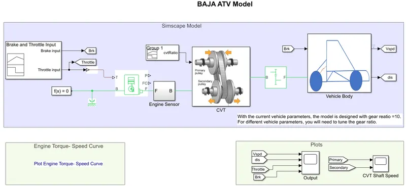
Above fig. is for BAJA ATV MODEL (Constant-Input). As can be seen there are three areas. Simscape Model, Engine Torque-Speed Curve & Plots.
`=>` Simscape Model Area :
Here the Simscape Model Area contains such blocks. Like Signal Builder, Generic Engine, Engine Sensor Subsystem, CVT (Continuously Variable Transmission) subsystem, Simple Gear & Vehicle Body Subassembly. Description of these blocks as per below.
`rarr` Signal Builder Block (Brake and Throttle Input) :
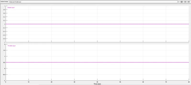
Using Signal Builder We are giving input for Brake & Throttle value. As per above. Where throttle value can be between 0 and 1.
`rarr` Generic Engine Block :
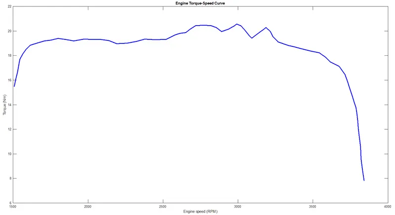
As per name Generic Engine block represents a general internal combustion engine. This block is a suitable generic engine for spark-ignition and diesel. Internal combustion engine with throttle and rotational inertia and time lag. The Generic Engine block uses a programmed relationship between torque and speed that is modulated by the throttle signal. Using 'T' port it takes thottle value where F and B are mechanical rotational conserving ports associated with the engine crankshaft and engine block, respectively. And based on the throttle value it take input of Speed vector & Torque vector values from given data of 'Engine Torque- Speed Curve' as per below can be seen.
`rarr` Engine RPM Sensor Subassembly :
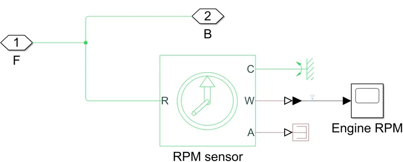
In this subassembly, Using 'Ideal Rotational Motion Sensor Block' RPM of engine is measured. And out value of RPM can be seen at the end of report. Inside the subassembly as below.
`rarr` CVT Subassembly :
CVT means Continuously_variable_transmission. Inside the subassembly as per below.
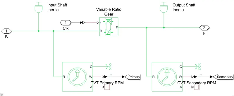
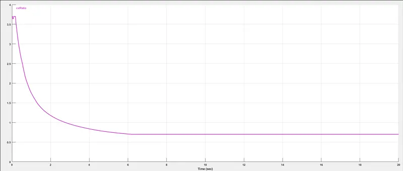
As can be seen from the above image using 'Variable Ratio Transmission Block' changing the RPM of the car This block's RPM-output based on 'cvt ratio' that is given with respect to time as below curve.(to match actual condition, otherwise we have to insert own ratio).
`rarr` Simple Gear Block :
Using this block we are reducing the 'Variable Ratio Gear' speed to a ratio of 10. Here the purpose of reducing speed is to increase the torque value with respect to vehicle tire diameter,weight and some other parameters are responsible.
`rarr` Vehicle Body Subassembly :
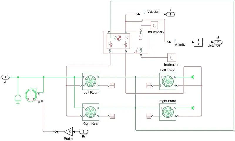
As above we can see what's inside the Vehicle Body Subassembly. Now Final speed is given to 'mechanical rotational conserving port A' of 'Tire Block'. Where this Final speed is given to both rear wheels only. Front both wheels are free to rotate as its 'A' port is attached with 'Rotational Free End Block'. Some more ports of 'Tire Blocks' are connected to 'Vehicle Body'.
The 'Vehicle Block' is Represents a two-axle vehicle body in longitudinal motion. The block accounts for body mass, aerodynamic drag, road incline, and weight distribution between axles due to acceleration and road profile. Where Connection H is the mechanical translational conserving port associated with the horizontal motion of the vehicle body. The resulting traction motion developed by tires should be connected to this port. Connections V, NF, and NR are physical signal output ports for vehicle velocity and front and rear normal wheel forces, respectively. In this Simulation wind resistance & Inclination resistance are taken 0. From the V port plotting the velocity & distance .
`=>` Engine Torque-Speed Curve Area : This contain an Engine Torque - Speed Curve Area Graph that we see in Above Description.
`=>` Plot Area : This contains Plot of Vehicle output like, Velocity, Distance, & Some input like, Throttle, Break. And Shaft speeds Primary/Secondary.
Let's see some output based on different input.
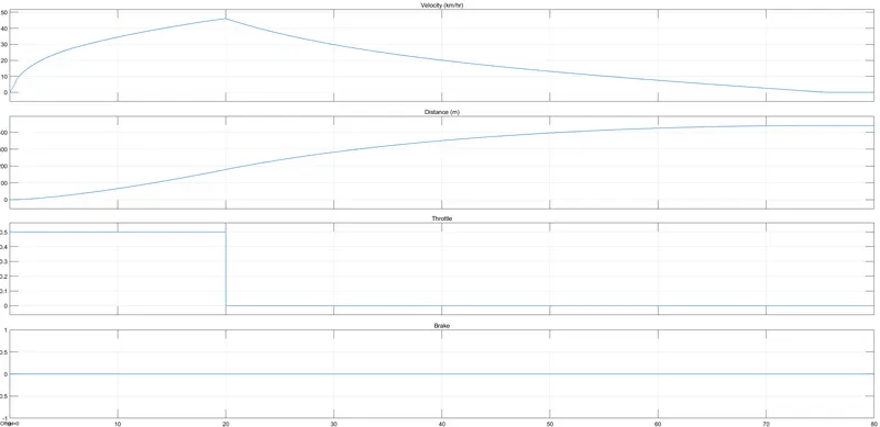
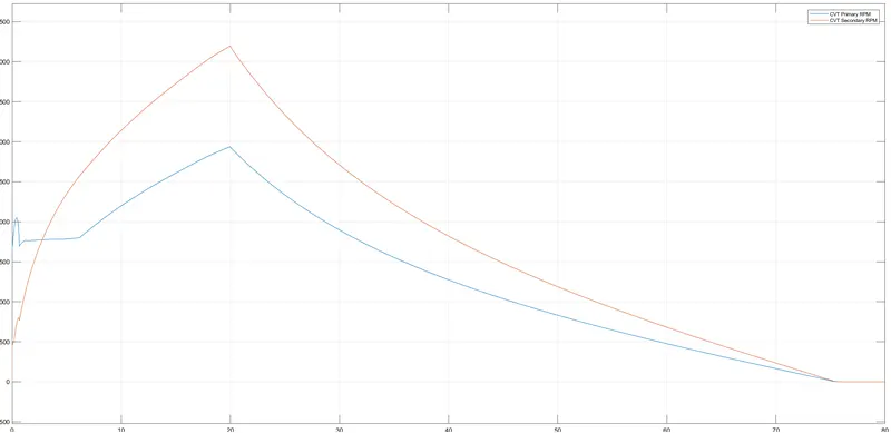
As below we can see how the Vehicle increases its speed from 0 to 45 km/h in 20 sec while throttle is applied. Then suddenly by stopping the throttle we can see how the vehicle gradually slows its speed. & From 'CVT Shaft Speed Plot' we can see how the gear ratio is changed with time. And on last Vehicle covered a 440m distance.
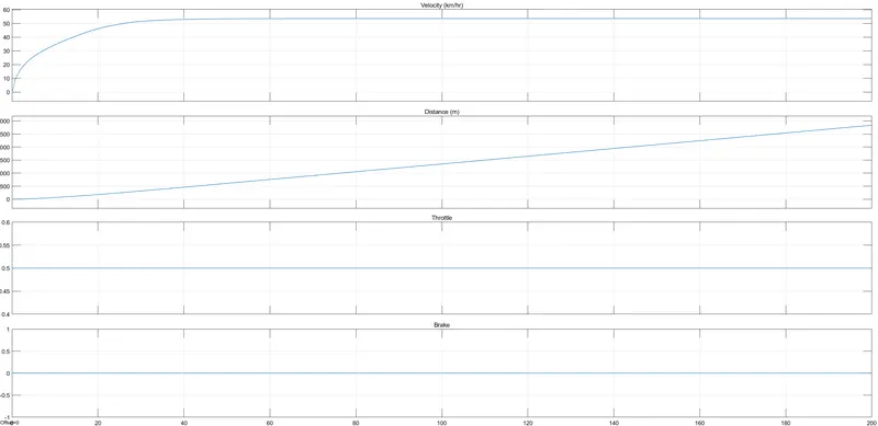
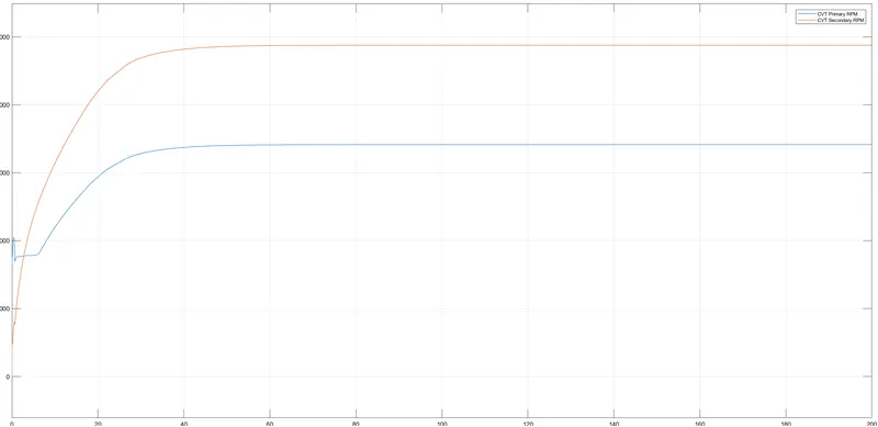
Now, We put the throttle constant all the time so based on that at a certain point vehicle speed should be constant. So we can see in the below graph that, 0-40sec vehicle covered it's top most velocity at 53 km/h and then constant. And For 200sec simulation vehicle covered almost 2800m dis.
`|><|` BAJA ATV MODEL (Variable-Input) :
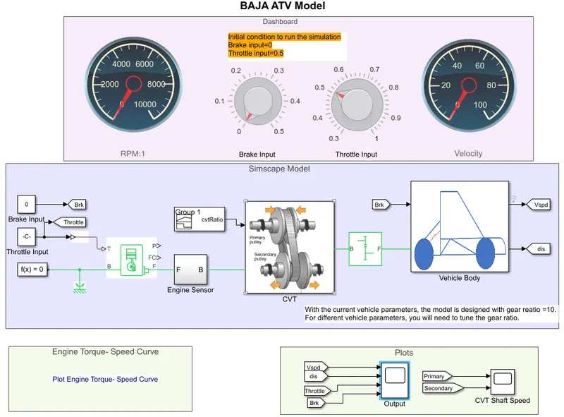
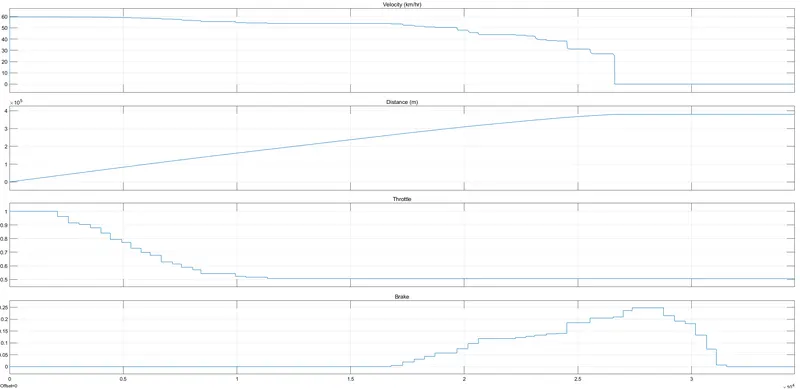
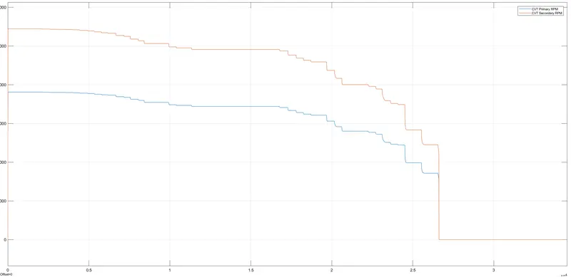
In Above screen we can see that all are the same, only the Dashboard area is added. Where using 'Knob block' we are giving variable input we respect to time. Real Time changes we can see from the 'Circular Gauge Block' RPM & Velocity. From below Graph we can see how using a variable input other parameters changes.
4. CONCLUSION:
By performing the above Project, I learn how any vehicle can be simulated in the Matlab Simulink environment. How actual vehicle data can be used as input. I learned some new blocks Such as, 'Generic Engine', 'Variable Ratio transmission', 'Tire', 'Vehicle Body' and many others.
REFERENCES :