Project
BAJA ALL Terrain (ATV) Simulink Model
Objective:
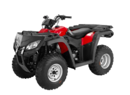
To perform a system-level simulation and analysis of a BAJA all-terrain vehicle (ATV) like the one shown in Figure 1, where select functional subsystems are modelled in Simulink to assess the performance of the ATV for predefined throttle, braking and CVT gearing schedules.
A detailed report is provided which describes the modelling concept and operation of the selected functional subsystems, and their role in the performance of the ATV.
Assumptions:
The following are the inferred assumptions for the BAJA ATV design project:
- There are no transmission, viscous or meshing losses
- The ATV is moving along and remains in contact with a level surface
- The wind speed is 0 km/hr
- Braking is not engaged during simulation
- All shafts rotate in the same direction as the crankshaft
- The ATV initiates operation when the crankshaft speed is at 1600 RPM
Figure 1. Picture BAJA ATV
Description:
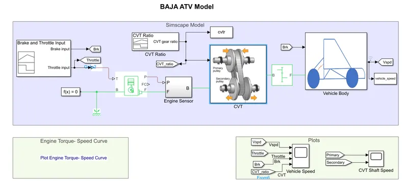
The BAJA ATV is composed of several functional subsystems that are modeled using appropriate Simulink and Simscape blocks. The selected functional subsystems considered in the Project facilitate the analysis of the translational and rotational dynamic performance of the ATV. These functional subsystems are as follows:
- Throttle
- Engine
- Engine Sensor
- Continuously Variable Transmission (CVT)
- Rear Wheel Differential
- Vehicle Body, Chassis and Wheels
- Braking
An overview of the BAJA ATV Simulink Model with the functional subsystems listed above is shown in Figure 2.
Figure 2. Simulink Model of select functional subsystems of the BAJA ATV
Throttle:
The Throttle is the functional subsystem used to set the torque required from the engine. The Throttle subsystem varies the throttle position from 0 through to 100%. Where, 0% throttle position represents zero torque required from the engine and 100% throttle represents a request for maximum torque from the engine based on its torque-speed capability. Throttle positions between 0 and 100% represent requests for the corresponding fractional value of the speed-dependent torque capability of the engine.
In the Simulink Model of the BAJA ATV, the Throttle subsystem is modelled using a Signal Builder block from the Simulink library with a predefined signal for the throttle input to the engine over the simulation period. In the first 20 seconds of the simulation, the throttle is set to a constant value of 0.3 (or 30%) and 1.0 (or 100%) for the rest of the simulation period as shown in Figure 3. Note that the engine responds to the defined throttle inputs based on the engine's torque-speed capability characteristics as shown in Figure 4. Observe that the initial portion of the curve in Figure 4 represents 30% throttle. In contrast, observe the torque-speed capability with 100% throttle for the entire simulation period in Figure 5.
Figure 3. Throttle schedule for BAJA ATV Project
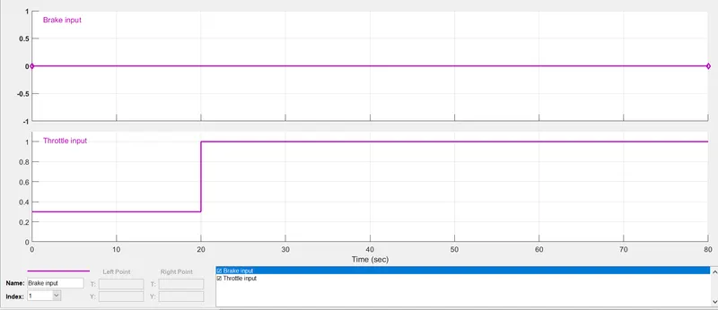
Figure 4. ATV Torque-speed performance at initial throttle of 30% with step to 100%
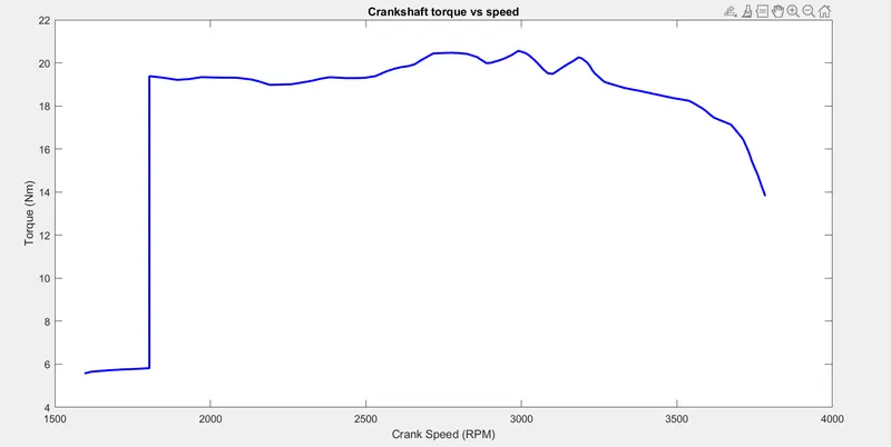
Figure 5. ATV torque-speed capability curve at 100% throttle
Engine:
The Engine is the functional subsystem that responds to requests from the Throttle subsystem. The Engine responds by developing the corresponding torque at the crankshaft (F) based on the throttle position.
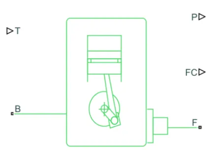
The BAJA ATV engine is modelled using a Generic Engine block from Simscape Driveline as illustrated in Figure 6. The Generic Engine model is used to describe the torque-speed capability of the ATV's engine by employing a torque vector and corresponding speed vector. Parameters such as the initial engine speed, inertia of the crankshaft and other engine performance constants are define defined in the Generic Engine model.
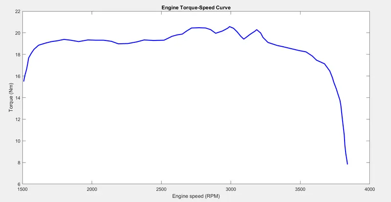
Vectors "speedVector" and "torqueVector" are used to describe the torque-speed capability of the ATV engine. The corresponding torque-speed capability curve is shown in Figure 5. In the analysis, the initial speed of the crankshaft is set to 1600 RPM at the start of the simulation with the inertia of the crankshaft set to 5 kgm^2. Note that the analysis of the engine fuel consumption is outside the scope of the analysis.
Per Figure 6, the T port of the Generic Engine model accepts the throttle position schedule. The B port represents the stationary part of the engine block and the F port represents the crankshaft. Note that the P port is used to access and monitor the power developed by the engine and the FC port used to access and monitor the fuel consumption of the engine.
Figure 6. Generic Engine Model use for BAJA ATV Engine
Engine Sensor:
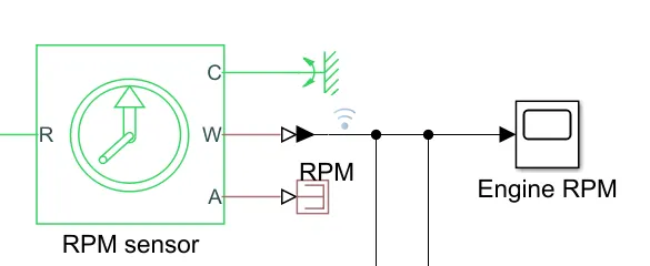
The Engine Sensor functional subsystem is used to monitor the speed of the crankshaft. A Simscape RPM Sensor (shown in Figure 7) interfaces with and is used to monitor the speed of the crankshaft over the period of the simulation.
A Simulink scope is connected to the speed port (W) of the RPM Sensor via a physical-Simulink signal converter. The Simulink scope captures the crankshaft RPM over the simulation period, however, an appropriate analog type measurement device from the Simulink Dashboard library (such as a Gauge) could also be used to monitor the RPM of the crankshaft over the simulation period. The stationary part of the RPM Sensor is connected to a fixed rotational reference frame via port C, which enables the correct outputs to be accessible from the W and A ports of the RPM Sensor.
Figure 7. Simscape RPM Sensor with Simulink Scope
Continuously Variable Transmission (CVT):
The CVT functional subsystem is used to continuously vary the transmission gear ratio in order to develop the appropriate torque at the wheels of the ATV thus managing its speed. The CVT functional subsystem is modelled using the Simscape blocks as shown in Figure 8.
The input and output shafts connected to the CVT are modelled using their corresponding mass moment of inertia values. The speeds of the input and output shafts are measured using Simscape RPM Sensors. The speeds of the input and output shafts are also monitored using two channels of a Simulink scope as shown in Figure 2.
A Variable Ratio Gear block is used to model the CVT. The Variable Ratio Gear block accepts a predefined signal from a Signal Builder block that represents the scheduled CVT gear ratio. The CVT gear ratio is defined as the ratio of the input shaft (B) speed to the output shaft (F) speed.
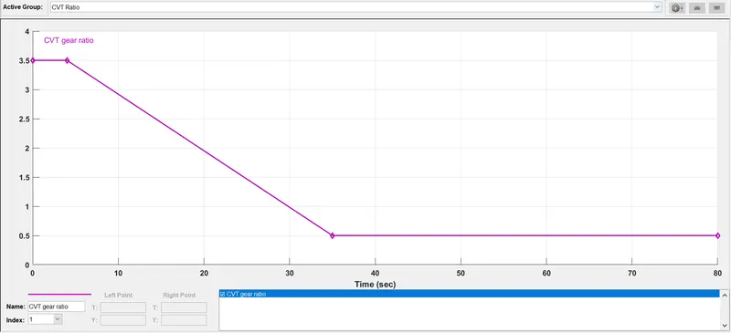
In the ATV CVT model, the predefined gear ratio has a scheduled starting value of 3.5, which is maintained for 4 seconds, after which the gear ratio falls linearly to 0.5 at 35 seconds. The CVT gear ratio is subsequently maintained at 0.5 for the rest of the simulation. The CVT gear ratio schedule is shown in Figure 10. The CVT gear ratio is copied to the workspace using a Simulink To Workspace block with variable name "cvtr".
The CVT gear ratio is correlated with the ATV's linear speed in the analysis in order to understand the relationship between the ATV's linear speed and the CVT gear ratio. As illustrated in Figure 9, the lower the CVT gear ratio the higher the linear speed of the ATV. So that a low CVT gear ratio is manifested when the speed of the output (secondary) shaft is greater than that of the input (primary) shaft and a high CVT gear ratio is manifested when the speed of the input (primary) shaft is greater than that of the output (secondary) shaft.
Observe that the CVT gear ratio starts at a value of 3.5 and decreases with time in the simulation. This is done to provide relatively high accelerating torque at the wheels of the ATV at the start of the simulation. As the linear speed of the ATV increases, the accelerating torque at the wheels is reduced by reducing the CVT gear ratio.
Figure 8. CVT gear ratio model with input and output shaft speed sensors
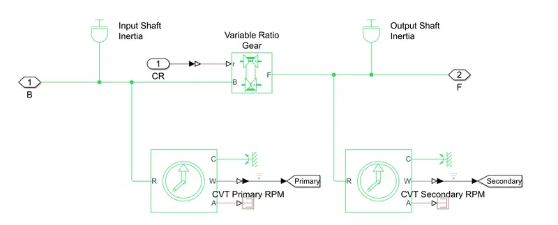
Figure 9. Relationship between CVT Ratio and ATV linear speed
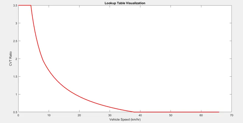
Figure 10. CVT gear ratio schedule
Rear Wheel Differential:
The Rear Wheel Differential functional subsystem connects the output shaft from the CVT to the rear wheels of the ATV. This subsystem transmits rotational energy to the rear wheels of the ATV using an appropriate gear ratio to meet the linear speed performance requirement of the ATV.
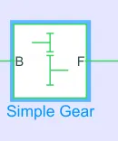
A Simscape Simple Gear block (per Figure 11) is used to model the Rear Wheel Differential, where the gear ratio is defined as the ratio of the number of teeth on the Follower Gear to that on the Base Gear. The Follower Gear rotates at the speed of the rear wheels of the ATV and the Base Gear rotates at the speed of the output shaft from the CVT. A fixed differential gear ratio of 12 is used in the analysis and no meshing or viscous losses are assumed.
Figure 11. Simple Gear Model Block
Vehicle Body Chassis and Wheels:
The Vehicle Body and Chassis (Figure 12) functional subsystem structurally houses all the components of the previously defined functional subsystems. The Vehicle body is mounted on the Chassis and both move together in a linear manner. Rotational energy in transmitted from the differential to the rear wheels and the front wheels are free to rotate in synch with the rear wheels. The rotation of the wheels transforms rotational energy to translational energy, hence the linear movement of the ATV.
The rotational and translational dynamics of the ATV are primarily dependent on the CVT gear ratio variation, total mass of the ATV, moment of inertia of the rotating components, net forces acting on the ATV body and chassis components, and net torque acting on the rotating components. Hence Newtonian translational and rotational differential equations that describe the ATV system can be developed and solved using Simulink. The solution of such equations provides information on rotational and translational quantities such as torque, forces, power, linear and angular speed, linear and angular acceleration, etc.
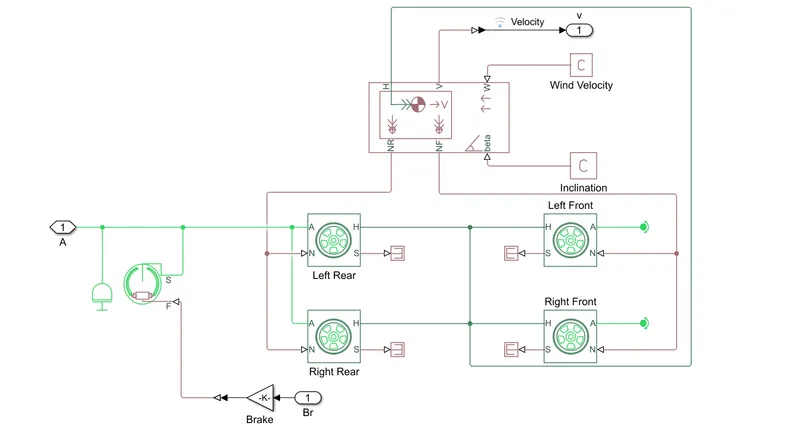
The Simscape model in Figure 13 is a symbolic block representation of the vehicle body, chassis, wheels and brakes. As illustrated in Figure 13, the vehicle body is subjected to wind resistance which is entered via the W port (modeled as zero in the analysis) and level of incline of the ATV, which is entered via the beta port (ATV on level surface). The vehicle body is connected to the four wheels via their H ports so that the vehicle body and wheels move linearly as one system.
Two wheels are modeled on each axle, that is, on the front and rear axles. The normal forces acting on the front and rear axles due to the mass and geometry of the vehicle body is accessible via ports NF and NR, respectively, on the vehicle body block. The normal forces are applied as inputs to the N port of the wheel blocks, which represent the normal forces acting downward on the tires, where equal forces act on the tires connected to the same axle. Torque from the output shaft of the differential is applied equally to the rear wheels via their A ports. Note that the slip port S of the tires are not monitored as shown in Figure 13.
Figure 12. ATV Vehicle Body Simplified Representation
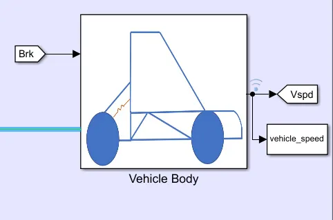
Figure 13. Detailed Model of Vehicle Body, Chassis and Wheels
Brakes:
The Brakes subsystem is used to apply an appropriate opposing torque to the rotating components of the ATV. This is done to decelerate the ATV. Typically, the Brake and Throttle subsystems are not engaged concurrently.
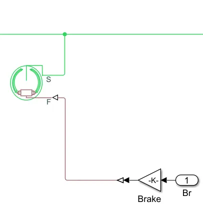
The Brake subsystem is modeled as shown in Figure 14, where a double-shoe brake Simscape block is used to represent the braking component. The double-shoe brake model has an F port that accepts a braking command from the Brake input of the Signal Builder block in Figure 2. A gain block is used to amplify the braking signal from the Signal Builder block by 1000 per Figure 14. The amplified signal is applied to port F of the double-shoe brake model. The S port of the double-shoe brake model is connected to the output shaft from the differential. Note that the braking subsystem is not engaged throughout the entire simulation period as shown in Figure 3. Thus, the braking subsystem does not play a significant role in the analysis.
Figure 14.
Analysis of Results:
Initial conditions
The pre-defined scheduled inputs to the BAJA ATV are:
- Throttle and Brake inputs (per Figure 3)
- The CVT gear ratio (per Figure 10)
The initial speed of the crankshaft at the start of the simulation is 1600 RPM as parameterized on the Dynamics tab of the Generic Engine model. However, the initial speed of the ATV is 0 km/hr at the start of the simulation as parameterized on the Dynamics tab of the wheel models.
Discussion
The plot in Figure 15 shows the speed of the ATV over the simulation period as the Throttle and CVT gear ratio changes with time.
Based on the initial throttle position of 0.3 and CVT gear ratio of 3.5, observe that the ATV quickly accelerates from 0 km/hr to 4 km/hr in approximately 104 ms as shown in Figure 16. Per Figure 17, the ATV speed remains at 4 km/hr up to 4 seconds and steadily increases thereafter due to the linear decrease in the CVT gear ratio, while the throttle remains at 0.3.
At 20 seconds, the throttle position changes to 1.0 (full throttle) while the CVT gear ratio continues to decrease. This results in an exponential increase in the speed of the ATV, which attains a speed of 38 km/hr at 35 seconds. After 35 seconds, the CVT gear ratio remains constant at 0.5 and the throttle also remains constant at 1.0. This results in a reduction in the acceleration of the ATV, with the ATV reaching a steady state speed of 65 km/hr at approximately 140 seconds as illustrated in Figure 18.
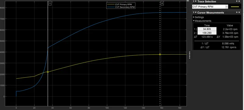
As illustrated in Figure 19, the trajectory of the CVT Secondary shaft RPM is consistent with that of the ATV's linear velocity. This is due to the fixed differential gear ratio. Observe that the minimum CVT gear ratio is selected such that the speed of the crankshaft and the Primary CVT shaft do not exceed 38397 RPM, which is the speed limit of the ATV's engine torque-speed capability curve.
Observe in Figure 19 that the acceleration of the CVT Primary shaft is not very sensitive to the changes in the throttle position and CVT gear ratio. The CVT Primary shaft RPM increases steadily from 1600 RPM. At 20 seconds, the acceleration of the CVT Primary shaft increases incrementally due to the change in throttle position to 1.0. When the throttle position remains constant at 1.0 and the CVT gear ratio at 0.5, the acceleration of the CVT Primary shaft decreases incrementally. Observe that the CVT Primary shaft reaches a steady-state speed of 3780 RPM at 140 seconds.
Figure 15. ATV linear speed over simulation period
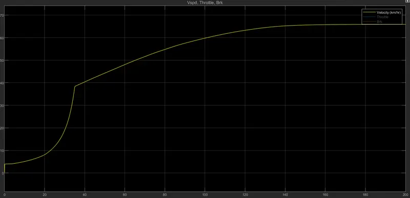
Figure 16. Initial ATV linear acceleration
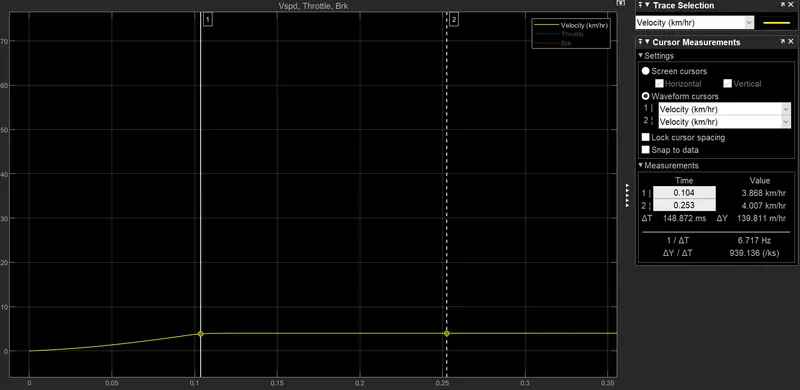
Figure 17. Speed performance compared with throttle position and CVT gear ratio
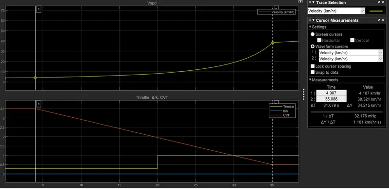
Figure 18. Steady-state ATV linear speed performance up to and after 140s
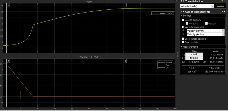
Figure 19. CVT Primary and Secondary shaft Speed Performance
Conclusion
The results of the analysis for the BAJA ATV project demonstrates that if the design assumptions are true; the model parameterization of the functional subsystems is correct and; the CVT gear ratio is operated no less than 0.5, then the BAJA ATV built per design should achieve a top speed of 65 km/hr on a level surface with no head wind.