Project
Aim:
To write a technical report on the simulation of a BAJA All-Terrain Vehicle (ATV) under various situations.
Objectives:
Perform a system-level simulation of an all-terrain vehicle and write a technical report that explains the model properties and provides feedback on the results.
ALL TERRAIN VEHICLE:
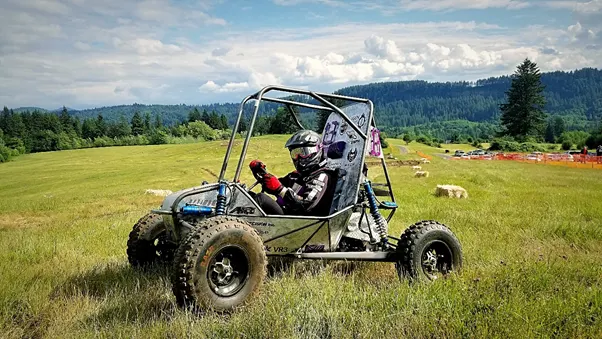
An all-terrain vehicle (ATV) is a motorised off-highway vehicle with four low-pressure or non-pneumatic tyres, a seat meant to be straddled by the operator, and handlebars for steering control. It also features a transmission, which transfers power from the engine to the wheels via shafts. It is divided into four categories. Manual transmission, continuously variable transmission, and semi-automatic transmission are the most common.
Automatic transmission
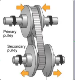
A CVT is a form of automatic transmission that gives more usable power, better fuel economy, and a smoother driving experience than a typical automatic transmission. The CVT is a mechanism that allows the gearbox ratio to be varied step less without interrupting torque delivery. As a result, there are an endless number of ratios (between a minimum and maximum value). It is a gearless, automatic gearbox with a single speed that can shift through an endless number of gear ratios. The ability to effortlessly shift across these multiple gears provides a number of advantages, including incredibly smooth shifts and excellent fuel economy. A CVT extracts maximum engine power from a compact engine, allowing drivers to accelerate more quickly than traditional automatic transmissions. CVTs emit lower emissions due to their increased capacity to manage the engine speed range. CVTs are also lighter than conventional automatic transmissions.
Simulink blocks which are used in model.
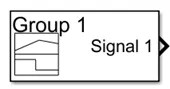
Signal builder
The signal builder creates the input signal required for the brake input, throttle input, and CVT gear ratio conditions. The signal is sent to the ATV vehicle by the signal builder. Using the signal builder, we produced our own signal for the 1980s. The signal for brake input and throttle for the engine is delivered to the generic engine via the signal building, which determines the engine performance. The CVT gear ratio generates the signal for the variable gear ratio block, which controls vehicle speed.
Generic engine
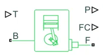
The generic engine receives input from the throttle signal and operates as expected (T). The mechanical reference block (B) is attached to the engine case (B). The crankshaft (F) turns in response to the throttle input (fuel signal) and is coupled to the sensor. The generic engine runs with predefined torque, speed, inertia, and so on.
Ideal rotational motion sensor
This sensor detects the rotation of the engine shaft. This sensor outputs velocity (W) and angular displacement (A). The velocity is converted to engine rpm and displayed in the scope. It is also used to calculate the rpm of the primary and secondary shafts.
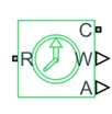
Mechanical rotational reference
The mechanical rotating reference can also be linked anywhere in the mechanical circuit when rotational-related components are utilised, the mechanical rotational reference must be attached. Used in conjunction with an ideal rotational motion sensor.

Simple gear
It is a fixed-ratio gearbox, and it changes the speed to a specific level. This block can also modify the speed's direction.
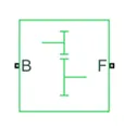
Variable ratio gear
The CVT transmission is used by the variable-ratio gear block. The block receives input from the gear ratio signal builder and causes the follower to run in accordance with the base. The ideal rotational sensor is used to measure the speed variations of the base and follower, and the values are displayed in the scope.
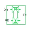
Finally, the shaft is linked to the vehicle body subsystem.
Inertia
The inertia block is used to provide mechanical rotational inertia by attaching to the shaft. This inertia causes the shaft's speed to vary slowly.
VEHICLE BODY SUBSYSTEM
The vehicle body block is made up of a vehicle body block, a tyre, and a double-shoe brake.
VEHICLE BODY BLOCK
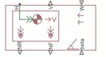
We can specify the vehicle mass, the number of axles per wheel, the distance of the axle from the centre, the height of the vehicle, wind velocity, the tilt of the vehicle, and so on using this block. The parameters are given constant values. Port(H) is connected to the mechanical translation component, Port(v) is connected to the vehicle's velocity, Port(W) is connected to the wind constant, Port(beta) is connected to the vehicle's inclination, Port (NF) is connected to the front tyres, and Port (NR) is connected to the rear tyres.
DOUBLE-SHOE BRAKE
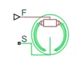
The signal builder's break input is connected to a double-shoe brake with a gain of 1000. The opposite end of the double-shoe brake is attached to the rotating shaft; as the input value is increased, the brake slows the speed of the shaft.
TIRE:
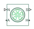
This block symbolises the vehicle's tyre. We can specify inertia, stiffeners, damping, and so on. Port(N) is connected to the physical signal input, Port(S) to the physical output, Port(H) to the mechanical translational, and Port(A) to the mechanical rotational. The magic formula depicts the tire's B-stiffness, C-shape, D-peak, and E-curvature.
SCOPE:-
It shows the signal that was generated during simulation.

Simulink – PS converter: -
Before providing input to the circuit, the signal from the source is transformed into a physical signal.
Ps Simulink converter: -
It converts the Input Physical Signal to a Simulink output signal.
Solver configuration: -
It defines solver settings to use for simulation.

Constant: - The constant block generates a constant value signal that might be real or complex. This block is used to give a steady signal input. Depending on the model, the block generates scalar, vector, or matrix output.

Integrator: -
The time derivative of the state is fed into the Integrator block. Using the current input value and the state value from the previous time step, the currently selected solver computes the output of the Integrator block at the current time step.

STUDY 1:
cvt model without dashboard
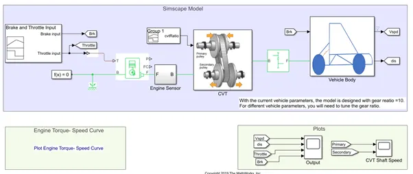
DESCRIPTION:
Initially, a signal builder is employed to provide the system with brake and throttle input. Go to blocks are used to transfer signals from blocks with the specified tag to other blocks. The signal generated by the signal builder is shown below.
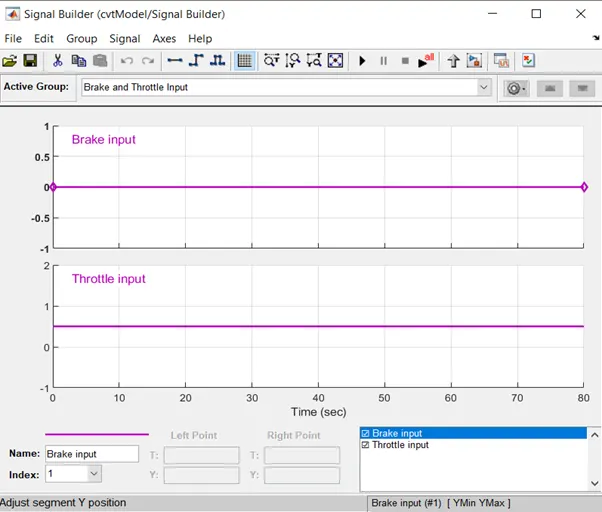
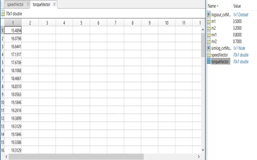
There is no break input offered here, but a throttle input is provided. The throttle setting is 0.3 for the first twenty seconds and one for the rest of the time. This output is then passed to a generic engine block that represents a system level model. The throttle input signal T, which ranges from 0 to 1, defines the torque needed from the engine as a percentage of the maximum available torque. Mechanical rotational conserving ports related with the engine crankshaft and engine block are represented by connections F and B, respectively. Connections P and FC are physical signal output ports used to report engine power and fuel consumption rate. The speed and torque vectors utilised in this block are obtained externally from the workspace.
This block is connected to a sub system named engine sensor. It is represented below.
R and C are mechanical rotational conserving ports and connectors of an ideal mechanical rotational motion sensor (RPM Sensor). W and A are velocity and angular displacement physical signal output ports, respectively. This is linked to a simple gear block, which is followed by CVT and car body subsystems. It is provided below.
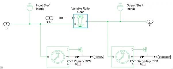
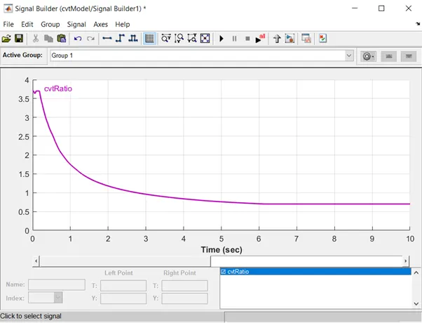
The workspace provides data for the input and output shaft inertias (m1 = 3.5 and m2 = 3.2) utilised in the CVT subsystem. A variable ratio gear receives these inputs. It denotes a variable ratio gearbox, such as those used in mechanical belt CVTs, electric transmissions, or hydraulic transmissions. The physical signal input r specifies the angular shaft velocity ratio between the input and output. Mechanical rotational conserving ports are connections B (base) and F (follower). With the Output shaft rotates parameter, you can specify the relationship between the rotation directions of the base and the follower. To detect the motion of two shafts, two rotational motion sensors are provided. Connections Rand Care and Wand A are mechanical rotational conserving ports and physical signal output ports for velocity and angular displacement, respectively. To provide gear ratio inputs to the CVT subsystem, a signal builder is used. It is depicted below.
As we said earlier, there is a vehicle body subsystem also. Its model is given below.
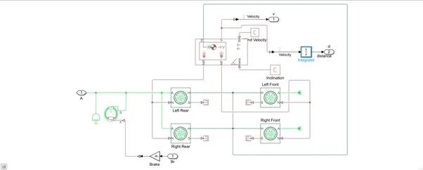
The major block in the vehicle body subsystem is the vehicle body block. It depicts a two-axle vehicle body moving longitudinally. Connection H is the mechanical translational conserving port linked with the vehicle body's horizontal motion. This port should be connected to the traction motion produced by the tyres. Physical signal output ports for vehicle velocity and front and rear normal wheel forces are represented by connections V, NF, and NR, respectively. When acting downhill, wheel forces are termed positive. Connections W and beta are physical signal input ports that correlate to the speed of the headwind and the angle of the road, respectively. The physical signal input ports CG and Mare are exposed if changing mass is modelled. CG takes a two-element vector with the x and y distance offsets between the vehicle CG and the additional load mass CG. M denotes the increased mass. When both variable mass and pitch dynamics are present, the physical signal port J accepts the additional mass's inertia about its own CG.
The tyres are then attached to a break drum block. It depicts a brake composed of two pivoted stiff shoes mounted symmetrically inside or outside a drum and actuated by a single actuator. The actuator force causes the shoes to apply friction torque to a shaft linked to the drum. Connections is a rotational terminal that conserves energy and is connected to the drum shaft. Connection F is a physical signal port that represents the actuator's force input. Positive force generates friction torque, which prevents the shaft from rotating. Its specifications are shown below.
Result
The scope results are shown below for cvtModel
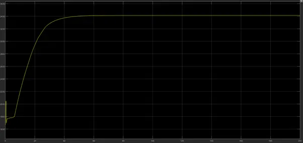
The above signal represents the engine rpm
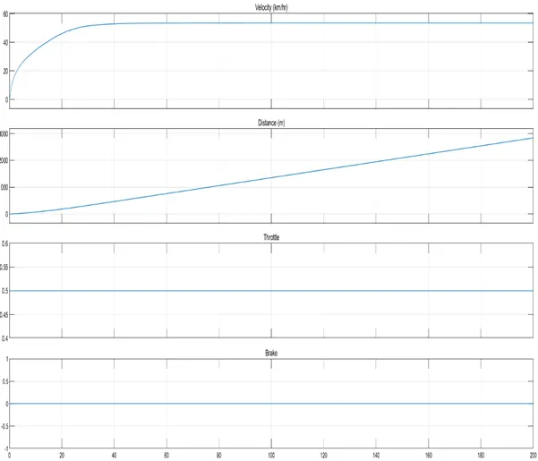
The above signal represents the velocity, throttle and brake.
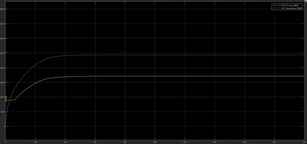
This plot depicts the variation in CVT shaft RMP and Secondary RPM during a 200-second period. The Simulink model is supplied after conducting several calculations to provide an appropriate result. As a result, a technical report explaining.
Study 2
cvt model with dashboard
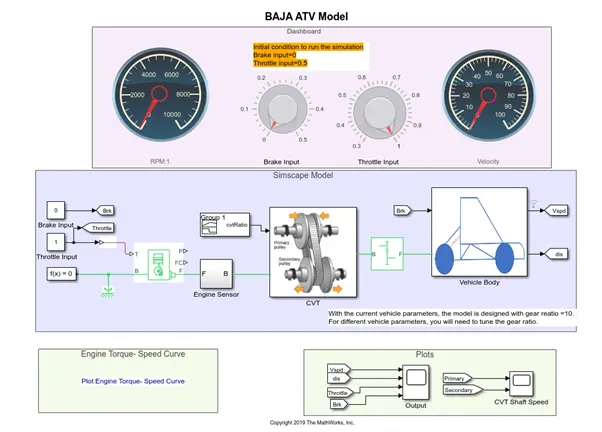
This model is identical to the CVT model; however, the input is provided through the dashboard control knobs. As a result, the throttle and brake input knobs are linked to the constant block, which gives input while the model runs indefinitely. This allows us to generate several scenarios while the simulation is running.
Blocks added
Circular Gauge: - to display the velocity and the RPM input.
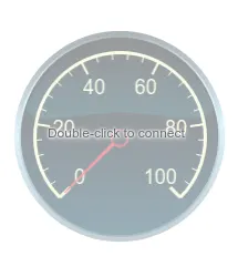
Knob: - to change input parameters.
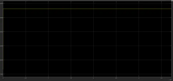
Result: -
We can see that the rpm remains constant at 3800 because the throttle input is constant and no brake is applied.
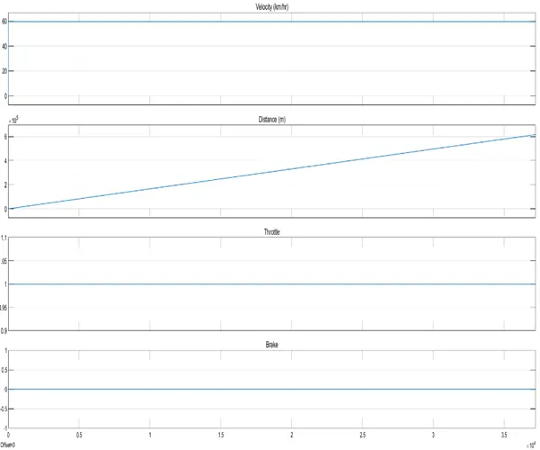
The above signal represents the velocity, throttle and brake.
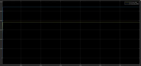
Shaft speed also behaved like previous case. Influence of break input brought down the maximum values and jerk was observed in the start.
Modelling with the help of LOOKUP TABLE
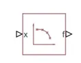
Lookup table blocks use data arrays to approximate mathematical functions by mapping input values to output values. In this case, we're going to use a PS lookup table (1D) block. It computes an approximation to a function given a set of data vectors. Physical signals will be used for both input and output. This model's data vectors are all the same length, and the x data vector is monotonic. The block then produces output based on the input values. We may also visualise the data prior to running the simulation. The lookup data visualisation is performed in this model, and the result is as follows.
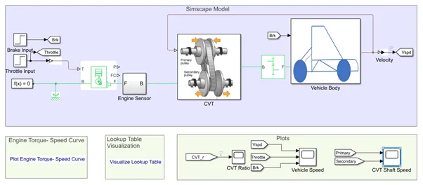
The sole difference between this model and the previous one is that the break and throttle inputs are given as step block values, and the CVT ratio is given via a lookup table block. The step time in the break input is 35, while the step time in the throttle input is 20. In prior circumstances, the CVT subsystem received the gear ratios as signals via signal building blocks. Lookup tables are used to provide the gear ratios in this case. A PS lookup table block is added to the CVT subsystem to do this. The simulation is now complete, and the results are presented below.
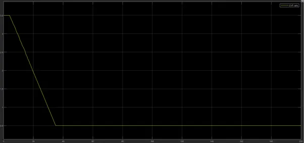
As we can see from the CVT Ratio plot, the value reduced from 2.3 to 1.8 when the speed exceeded 30. It remained consistent after that. Because we use step input, the drop is pretty straight. We can now investigate vehicle speed for more information.
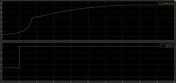
When the throttle was set to 1, the vehicle's speed unexpectedly rose after 20 seconds and reached over 55km/h. Shaft speed is depicted below.
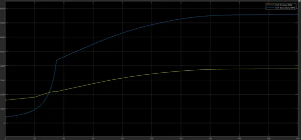
We can see that the shaft speed closely resembles the plot with the same type of throttle input. We may now examine the model's conditions using the dashboard.
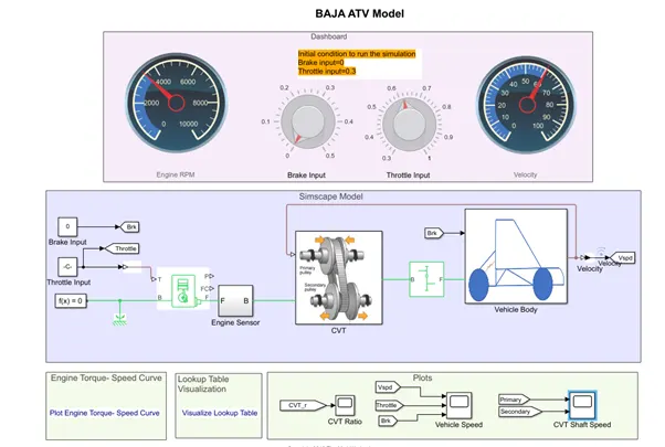
The dashboard in this case is outfitted with two knobs and two unique gauges. The knobs control the break and throttle, while the gauges display the velocity and rpm. Similarly, to the previous model, the CVT system has a lookup table block where we can enter gear ratios. We obtained the results after conducting the simulation, which are shown below.
Results
We start with the initial condition provided and will change accordingly.
Throttle input = 0.6 and Break input = 0
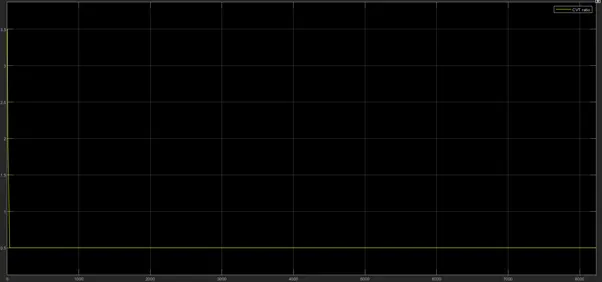
The CVT Ratio plot is shown above. We can see that the value abruptly shifted to a constant value of 0.5 when the simulation was run with a 0.6 throttle input.
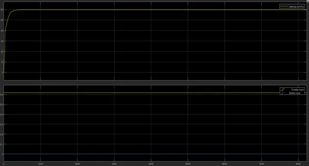
As the throttle input was steady, the vehicle speed remained constant at around 45km/h. As a result, the shaft speed was also constant, as shown below.
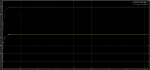
We can observe that, shaft speed exactly resembles the plot which have same kind of throttle input. Now we can check out the conditions for model with dashboard.
- BAJA ATV with Dashboard
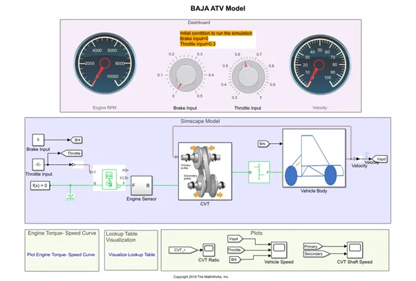
The dashboard in this case is made up of two knobs and two bespoke gauges. The knobs control the break and throttle, while the gauges display the velocity and rpm. Similarly, to the previous model, the CVT system has a lookup table block where we can enter gear ratios. We obtained the results after conducting the simulation, which are shown below.
Results
We start with the initial condition provided and will change accordingly.
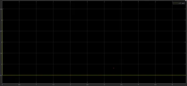
The CVT Ratio plot is shown above. We can see that the value abruptly shifted to a constant value of 0.5 when the simulation was run with a 0.6 throttle input.
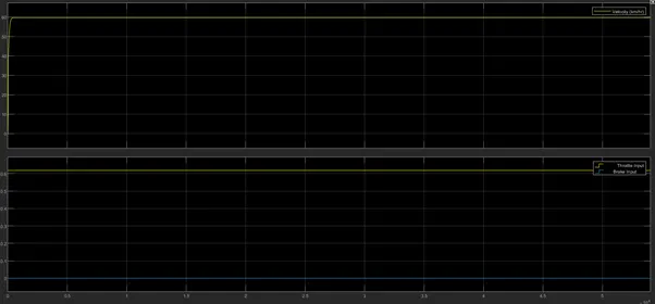
Vehicle Speed was constant at about 45km/hr as the throttle input was constant. So, the shaft speed was also constant and it is represented below.
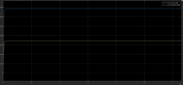
Each shaft is constant.
Conclusion:
The simulation analysis aids in understanding the change in concerned parameters with respect to the given inputs for distinct scenarios. Simulink allows us to analyse various simulations without creating code and simply by understanding how they work logically. The ATV BAJA Vehicle Analysis assists in examining the performance of vehicle metrics such as RPM, vehicle speed, Torque, gear ratio, and so on.