Project

Aim: To carry out a system-level simulation of an all-terrain vehicle (Baja) using Simulink.

Theory:

An all-terrain vehicle (ATV), also known as a light utility vehicle (LUV), a quad bike, or simply a quad, as defined by the American National Standards Institute (ANSI); is a vehicle that travels on low-pressure tires, with a seat that is straddled by the operator, along with handlebars for steering control. As the name implies, it is designed to handle a wider variety of terrain than most other vehicles. Although it is a street-legal vehicle in some countries, it is not street-legal within most states, territories, and provinces of Australia, the United States or Canada.

By the current ANSI definition, ATVs are intended for use by a single operator, although some companies have developed ATVs intended for use by the operator and one passenger. These ATVs are referred to as tandem ATVs.

The rider sits on and operates these vehicles like a motorcycle, but the extra wheels give more stability at slower speeds. Although most are equipped with three or four wheels, six-wheel models exist for specialized applications. Multiple-user analogues with side-by-side seating are called utility terrain vehicles (UTVs) or side-by-sides to distinguish the classes of vehicle. Both classes tend to have similar powertrain parts. Engine sizes of ATVs are in the range from 49 to 1,000 cc (3.0 to 61 cu in).

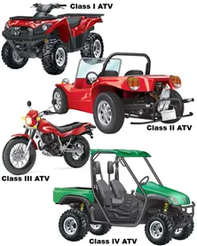
Components of Baja ATV:

Engine:

The most used engines for Baja ATVs are Briggs and Stratton (1450 series) horizontal OHV engine of 305 cc, 4-stroke petrol engine with single cylinder. It has power of 10 bhp at 1750 engine rpm.

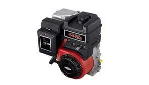
Continuously Variable Transmission (CVT):

A continuously variable transmission (CVT) is an automatic transmission that can change seamlessly through a continuous range of gear ratios. This contrasts with other transmissions that provide a limited number of gear ratios in fixed steps. The flexibility of a CVT with suitable control may allow the engine to operate at a constant RPM while the vehicle moves at varying speeds.

CVTs are used in automobiles, tractors, motor scooters, snowmobiles, and earthmoving equipment.

The most common type of CVT uses two pulleys connected by a belt or chain, however, several other designs have also been used at times.

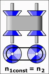
Body:

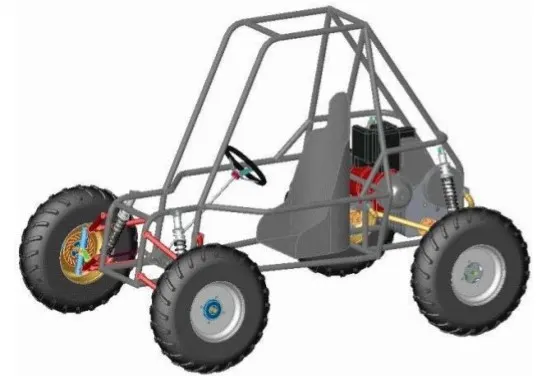
Body of Baja ATV consist of the following Components:

1. Frame/Chassis: The type of chassis used Baja ATV is roll cage chassis.
2. Steering System: The type of steering system used in Baja ATV is Ackerman Steering System
3. Braking System: The type of brakes used in Baja ATV is Double Shoe Brakes.
4. Drivetrain: Drivetrain contains components like Engine, CVT, Drive Shaft, Bearings, Hubs, etc.
5. Suspension: Shock Absorbers are used as suspension in Baja ATV.
6. Wheel assembly: Wheel Assembly contains Wheel Hubs, Bearings and Wheels.

System Level Simulation of Baja ATV using Simulink:

There are 2 Simulation of Baja ATV:

1. Simulation using Dashboard.
2. Simulation without using Dashboard.

Simulink Model for Simulation using Dashboard:

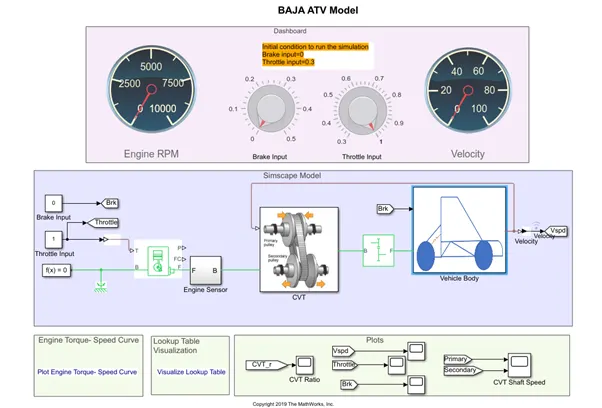
Dashboard:

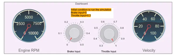
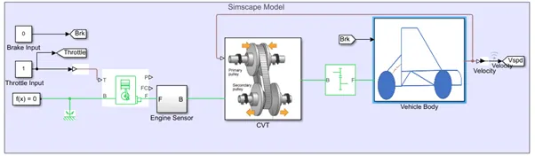
Here, the Brake and Throttle inputs are given by the user. The Brake input is from 0 to 0.5 and the Throttle input is from 0.3 to 1. This model can be run for infinite time and the user can change the values of Brake and Throttle inputs anytime.

Simulink Model for Simulation using Dashboard:

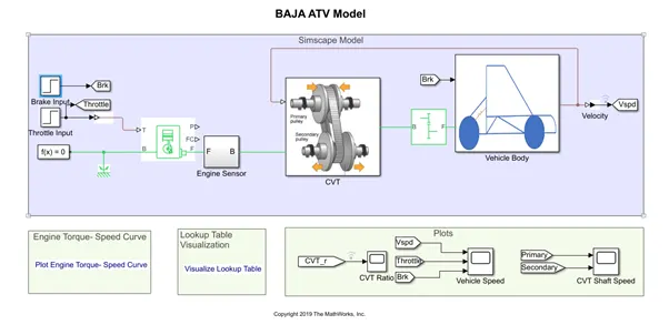
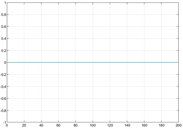
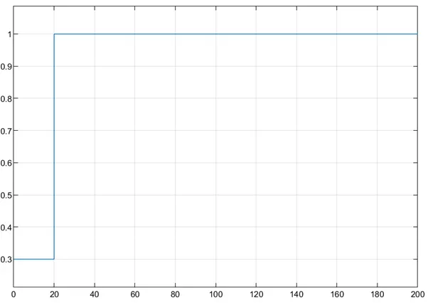
Here, the Brake and Throttle inputs are provided for 200 seconds by using the Step block. The following plots below are the Brake and Throttle inputs provided:

Brake input:

Throttle Input:

Simscape model:

(With Dashboard)

(Without Dashboard)

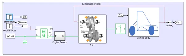
Here, we can see that the Brake and Throttle inputs are used for calculation for various part of the Baja ATV. We will see the calculation below:

Engine:

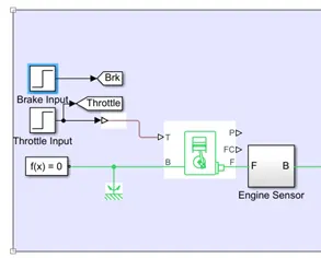
(With Dashboard) (Without Dashboard)

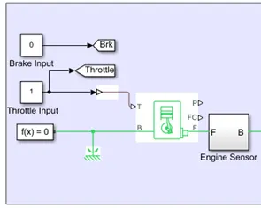
In the generic engine block, the Throttle input is the input given by the user in the dashboard. Connection B is connected to mechanical rotational reference as shown in the figure. The values for speed vector and torque vector are extracted from the following plot:

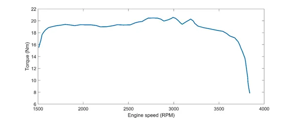
This data is extracted using the Grabit command in Matlab. Engine Power and Fuel Consumption of the engine is calculated and can be measured through the ports P and FC. The Engine Sensor subsystem is used to measure the Engine RPM which is connected to the port F of the generic engine block. The Engine RPM value is then used for the calculation of CVT.

CVT:

CVT Subsystem:

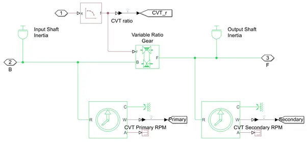
Here, Input and Output Shaft inertia represent primary and secondary pulley. A Variable Ratio Transmission block is used to change the speed of the Secondary Shaft as per the given plot below:

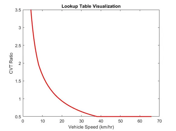
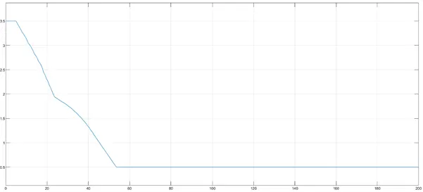
As we can see here, the CVT Ratio changes with change in velocity of the vehicle. The value of the vehicle speed is taken from the Vehicle Body Subsystem and the change in CVT Ratio w.r.t. velocity for Baja ATV is done using the PS Lookup Table (1D) block. The value of CVT Ratio is then used in Variable Ratio Transmission Block.

Simple Gear:

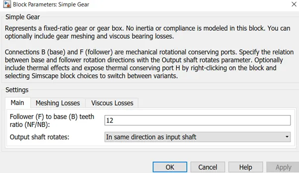
Here, a Simple Gear block is used for the reduction of speed. A gear ratio of 12 is used to reduce the speed of the CVT Shaft and the rear axle.

Usually, gear is used in between the generic engine and the CVT, so that to avoid any damage caused to CVT due to higher RPM values of generic engine.

Vehicle Body:

Vehicle Body Subsytem:

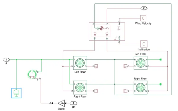
Here, we can see that the inertia block is connected to the signal from port A which represents the rear axle and then it is connected to Double-Shoe Brake block.

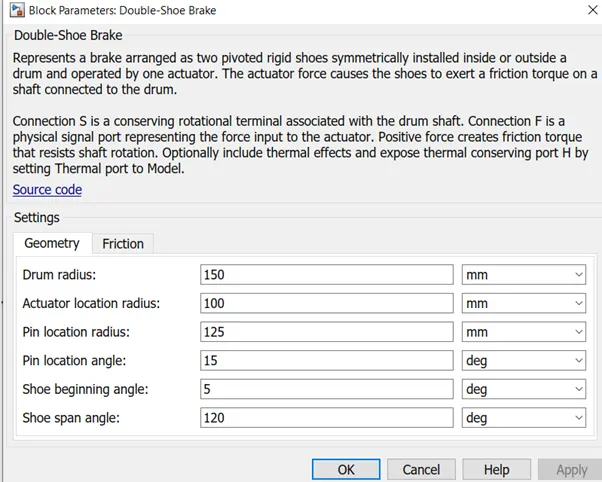
In the Double-Shoe brake block, the brake input given by the user or the values provided by the step block is multiplied by 1000 to convert into the force applied on the brake. The below table shows the various values allotted to the parameters of Double-Shoe Brake.

Tire:

Magic Formula:

Magic Formula, developed by Pacejka has been widely used to calculate steady-state tire force and moment characteristics. The semi-empirical tire model combined slip situation from a physical view point. The pneumatic trail is introduced as a basis to calculate this moment about the vertical axis.

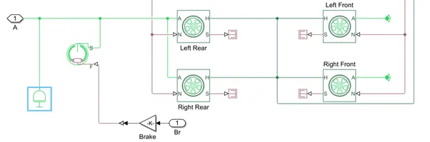
As we can see that the connection A (which is the mechanical rotational conserving port for the wheel axle) of the rear wheels (left and right) is connected to the Double-Shoe Brake and Port A (which is the signal coming from CVT), the thrust due to engine and braking effort due Double-Show Brake is applied on the rear wheels; while the port A of front wheels (left and right) is connected to rotational free end block due to the steering system connected to the front wheels.

Connection N is the normal force acting on the wheel due to the mass of the vehicle and Connection S is a physical signal output port that reports the tire slip. Connection H develops the thrust developed by the wheels and reports it to the vehicle body block.

Vehicle Body Block:

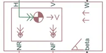
It represents a two-axle vehicle body in longitudinal motion. The block accounts for body mass, aerodynamic drag, road incline, and weight distribution between axles due to acceleration and road profile. The vehicle can have the same or a different number of wheels on each axle. Optionally include pitch and suspension dynamics or additional variable mass and inertia. The vehicle does not move vertically relative to the ground.

The values for various parameters of vehicle body and aerodynamic drag acting on the vehicle are shown in the table below:

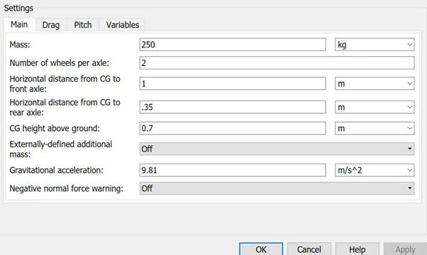
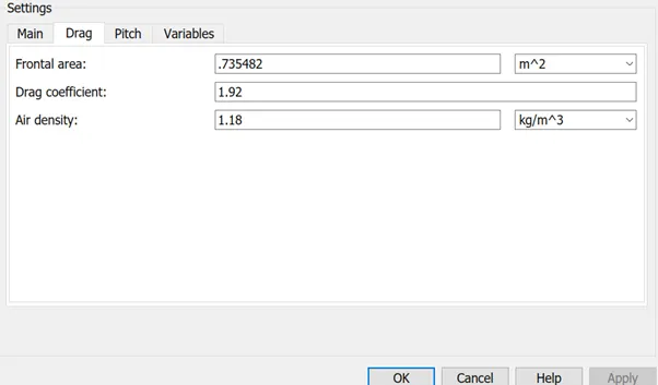
The final velocity of the vehicle is calculated in this block.

Results (With Dashboard):

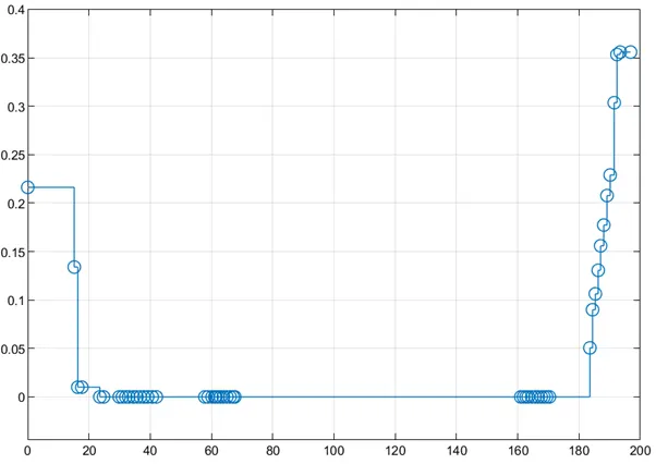
The simulation was run for 200 seconds with following Brake and Throttle user inputs:

Brake input:

Throttle Input:

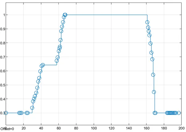
Here, Throttle was reduced at time around 170 second and Brake were applied.

Below is the velocity plot of the vehicle.

Velocity Plot:

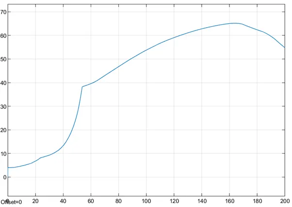
In this plot, we can see that the Throttle was increased gradually up to 170 seconds and Brake was applied after that and also the Throttle was reduced, due to which we can see that the velocity of the vehicle started to reduce after 170^th second.

Below are the plots for CVT Ratio, CVT Primary and Secondary Shaft Speeds and Engine Rpm:

CVT Ratio:

CVT Primary and Secondary Shaft Speeds:

Engine RPM:

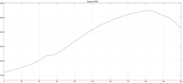
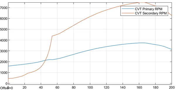
The drop in the RPM speeds after 170^th second is because of the reason mention in the velocity plot.

Results (With Dashboard):

The simulation was run for 200 seconds and the Brake and Throttle inputs give from the Step block is given below:

Brake input:

Brakes were not applied for the whole simulation process.

Throttle Input:

Throttle was applied from 0.3 to 1 at 20^th second.

Below is the Velocity plot of the vehicle:

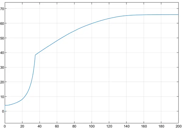
We can see that the Velocity was constant after the time around 150^th second because the Throttle input was constant of value 1 from 20^th second to 200^th second.

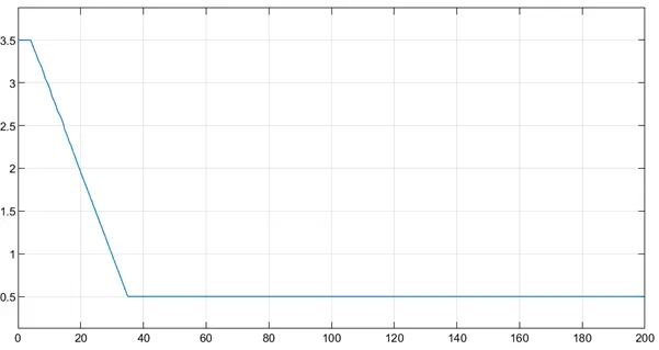
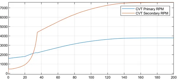
Below are the plots for CVT Ratio, CVT Primary and Secondary Shaft Speeds and Engine Rpm:

CVT Ratio:

CVT Primary and Secondary Shaft Speeds:

Engine RPM:

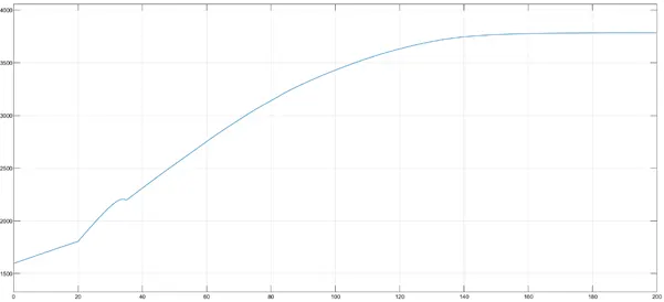
We can see that the RPM Values are constant after 150^th second because of the reason mention in the velocity plot.

We can also see in both simulations (with and without Dashboard) that the CVT Secondary Shaft RPM Speed starts from 500 RPM and the CVT Primary Shaft RPM Speed starts from 1500 RPM at the start of the simulation, but at the end of the simulation, we can see that the Secondary RPM is twice than the Primary RPM, it is because of the of the CVT Ratio which starts from 3.5 when the vehicle is at rest and it is 0.5 when vehicle reaches a speed of around 35 kmph.