Project 2 - Rankine cycle Simulator

Aim: To create a Rankine Cycle Simulator in Matlab by taking user inputs

Theory: There are 4 main processes in a Rankine Cycle

1. Process 1-2 is Isentropic Expansion in the Turbine:

Water is in the vapour form in the turbine, so the calculations are calculated by the vapour formulas like ‘hV_p’ and ‘sV_p’.

In this process, Pressure(p1) and Temperature(t1) are taken as user inputs and Enthalpy(h1) and Entropy(s1) are calculated using XSteam function.

2. Process 2-3 is Constant Pressure Heat Rejection in the Condenser:

Water is in the vapour form in the condenser, so the calculations are calculated by the vapour formulas like ‘hV_p’ and ‘sV_p’.

In this process, Pressure(p2) is user input and Enthalpy(s2) is equal to Enthalpy(s1). Temperature(t2) and Entropy (s2) can be calculated.

3. Process 3-4 is Isentropic Compression in the Pump:

Water is in the liquid form in the pump, so the calculations are calculated by the liquid formulas like ‘hL_p’ and ‘sL_p’.

In this process, Pressure(p3) is equal to pressure(p2) and Temperature(t3) is equal to temperature(t2). Enthalpy(h3) and Entropy(s3) can be calculated using XSteam function.

4. Process 4-1 is Constant Pressure Heat Addition by the Boiler:

Water is in the liquid form in the pump, so the calculations are calculated by the liquid formulas like ‘hL_p’ and ‘sL_p’.

In this process, Pressure(p4) is equal to pressure(p1) and Entropy(s4) is equal to Entropy(s3). Temperature(t4) and Enthalpy(h4) can be calculated.

Objectives:

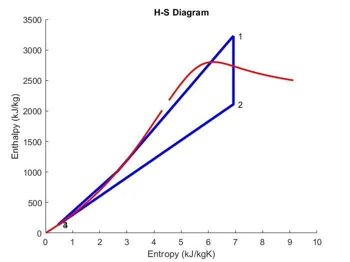
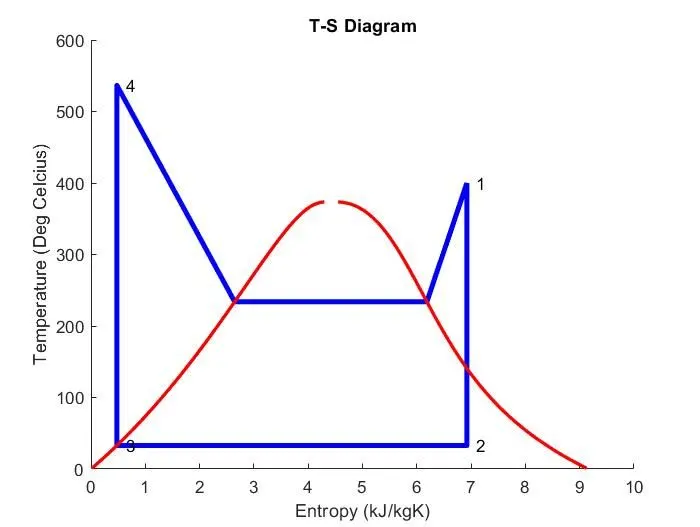
To take Pressure(p1,p2) and Temperature(t1) as user inputs and calculate net work output and basic work ratio and should also plot H-S and T-S graphs.

Program:

clear all 
close all
clc

%To display various process of rankine cycle
fprintf("Rankine Cycle Simulator\n");
fprintf("1-2 is Isentropic Expansion in the Turbine\n");
fprintf("2-3 is Constant Pressure Heat Rejection by the Condenser\n");
fprintf("3-4 is Isentropic Compression in the Pump\n");
fprintf("4-1 is Constant Pressure Heat Addition by the Boiler\n \n");

%To get user inputs of p1,t1,p2
p1 = input('Enter Pressure at Turbine Inlet(in Bar) = \n');
t1 = input('Enter the temperature at turbine inlet(in Degree Celcius) = \n');
p2 = input('Enter Pressure at the Condenser(in Bar) = \n');

t_sat_1 = XSteam('Tsat_p',p1);
if t_sat_1 <= t1
%Calculating and printing state point variables at state 1
%Enthalpy
h1 = XSteam('h_pT',p1,t1);
%Entropy
s1 = XSteam('s_pT',p1,t1);
fprintf("\nResults\n");
%Printing state 1 variables
fprintf("\nAt state point 1:\n");
fprintf('Pressure(P1) = %f Bar\nTemperaure(T2) = %f Deg Celcius\nEnthalpy(H1) = %f kJ/kg\nEntropy(S1) = %f kJ/kgK\n',p1,t1,h1,s1);

%Calculating and printing state point variables at state 2
%Entropy
s2 = s1;
p3 = p2;
%For Enthalpy and Temperature calculations
sg_2 = XSteam('sV_p',p2);
hg_2 = XSteam('hV_p',p2);
sf_3 = XSteam('sL_p',p3);
hf_3 = XSteam('hL_p',p3);
if s2 <= sg_2
    x2 = (s2 - sf_3)/(sg_2 - sf_3);
else
    x2 = 1;
end
t_sat_2 = XSteam('Tsat_p',p2);
cp2 = XSteam('CpV_p',p2);
if x2 < 1
    t2 = t_sat_2;
    h2 = hf_3+(x2*(hg_2-hf_3));
else
t2 = (t_sat_2 + 273)*exp((s2 - sg_2)/cp2);
%Temperarure
t2 = t2 - 273;
%Enthalpy
h2 = XSteam('hV_p',p2);
end
%Printing state 2 variables
fprintf("\nAt state point 2:\n");
fprintf('Pressure(P2) = %f Bar\nTemperaure(T2) = %f Deg Celcius\nX2 = %f\nEnthalpy(H2) = %f kJ/kg\nEntropy(S2) = %f kJ/kgK\n',p2,t2,x2,h2,s2);

%Calculating and printing state point variables at state 3
%Pressure

%Temperature
t3 = t2;
%Enthalpy
h3 = XSteam('hL_p',p3);
%Entropy
s3 = XSteam('sL_p',p3);
%Printing state 3 variables
fprintf("\nAt state point 3:\n");
fprintf('Pressure(P3) = %f Bar\nTemperaure(T3) = %f Deg Celcius\nEnthalpy(H3) = %f kJ/kg\nEntropy(S3) = %f kJ/kgK\n',p3,t3,h3,s3);

%Calculating and printing state point variables at state 4
%Pressure
p4 = p1;
%Entropy
s4 = s3;
%For Enthalpy and Temperature calculations

sf_4 = XSteam('sL_p',p4);

hf_4 = XSteam('hL_p',p4);
sg_4 = XSteam('sV_p',p4);
t_sat_4 = XSteam('Tsat_p',p4);
cp4 = XSteam('CpL_p',p4);
%Temperature
t4 = (t_sat_4 + 273)*exp((sg_2 - sg_4)/cp4);
t4 = t4 - 273;  
%t4 = t3;
%Enthalpy
v3 = XSteam('vL_p',p4);
wp = v3*(p4-p3)*100;
h4 = wp + h3;

%Printing state 4 variables
fprintf("\nAt state point 4:\n");
fprintf('Pressure(P4) = %f Bar\nTemperaure(T4) = %f Deg Celcius\nEnthalpy(H4) = %f kJ/kg\nEntropy(S4) = %f kJ/kgK\n',p4,t4,h4,s4);

%Vapour and Liquid line
T = linspace(1,t1,500);
for i = 1:length(T)
    Hv(i) = XSteam('hV_T',T(i));
    Hl(i) = XSteam('hL_T',T(i));
    Sv(i) = XSteam('sV_T',T(i));
    Sl(i) = XSteam('sL_T',T(i));
end

%Net work output and basic work ratio
wt = h1 - h2;
wnet = wt - wp;
qin = h1 - h4;
ntherm = (wnet/qin)*100;
ssc = 3600/wt;
fprintf('\nWt is = %f kJ/kg\nWp is = %f kJ/kg\nWnet is = %f kJ/kg\nNtherm is = %f percent \nS.S.C. is = %f kg/kWh',wt,wp,wnet,ntherm,ssc)

%plotting
figure(1)
hold on
plot([s1 s2 s3 s4 sf_4 sf_4 s1],[h1 h2 h3 h4 hf_4 hf_4 h1],'linewidth',3,'color','b')
text(s1,h1,'  1')
text(s2,h2,'  2')
text(s3,h3,'  3')
text(s4,h4,'  4')
plot(Sl,Hl,'linewidth',2,'color','r')
plot(Sv,Hv,'linewidth',2,'color','r')
xlabel('Entropy (kJ/kgK)')
ylabel('Enthalpy (kJ/kg)')
title('H-S Diagram')
figure(2)
hold on
plot([s1 s2 s3 s4 sf_4 sg_4 s1],[t1 t2 t3 t4 t_sat_4 t_sat_1 t1],'linewidth',3,'color','b')
text(s1,t1,'  1')
text(s2,t2,'  2')
text(s3,t3,'  3')
text(s4,t4,'  4')
plot(Sl,T,'linewidth',2,'color','r')
plot(Sv,T,'linewidth',2,'color','r')
xlabel('Entropy (kJ/kgK)')
ylabel('Temperature (Deg Celcius)')
title('T-S Diagram')

%if temperature input is below saturation temperature
else 
    fprintf('Enter Temperature greater or equal to saturation temperature %f Deg Celcius',t_sat_1)
end

Output:

Rankine Cycle Simulator
1-2 is Isentropic Expansion in the Turbine
2-3 is Constant Pressure Heat Rejection by the Condenser
3-4 is Isentropic Compression in the Pump
4-1 is Constant Pressure Heat Addition by the Boiler
 
Enter Pressure at Turbine Inlet(in Bar) = 
30
Enter the temperature at turbine inlet(in Degree Celcius) = 
400
Enter Pressure at the Condenser(in Bar) = 
0.05

Results

At state point 1:
Pressure(P1) = 30.000000 Bar
Temperaure(T2) = 400.000000 Deg Celcius
Enthalpy(H1) = 3231.571027 kJ/kg
Entropy(S1) = 6.923259 kJ/kgK

At state point 2:
Pressure(P2) = 0.050000 Bar
Temperaure(T2) = 32.875490 Deg Celcius
X2 = 0.814256
Enthalpy(H2) = 2110.708212 kJ/kg
Entropy(S2) = 6.923259 kJ/kgK

At state point 3:
Pressure(P3) = 0.050000 Bar
Temperaure(T3) = 32.875490 Deg Celcius
Enthalpy(H3) = 137.765119 kJ/kg
Entropy(S3) = 0.476254 kJ/kgK

At state point 4:
Pressure(P4) = 30.000000 Bar
Temperaure(T4) = 536.705747 Deg Celcius
Enthalpy(H4) = 141.409137 kJ/kg
Entropy(S4) = 0.476254 kJ/kgK

Wt is = 1120.862815 kJ/kg
Wp is = 3.644018 kJ/kg
Wnet is = 1117.218797 kJ/kg
Ntherm is = 36.154054 percent 
S.S.C. is = 3.211811 kg/kWh>> 

Plots: