Project 2 Thermal modeling of battery pack
Aim: To build a 10-cell series lithium-ion battery model, simulate the thermal effects and compare life cycle performance at various temperatures, charge & discharge rates using MATLAB.
Solution:
A simple thermal model is used to model battery temperature. It is assumed that heating is primarily from internal resistance and that cooling is primarily via convection.
A 10-cell series lithium-ion battery pack can be modeled by connecting multiple copies of the battery cell block in series.
We will continue with the existing Simulink model example which is present on Mathworks.com,
" Lithium-Ion Battery Pack with Fault "
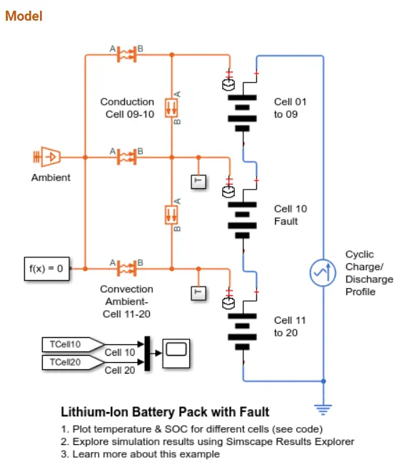
This example shows how to simulate a battery pack consisting of multiple series-connected cells in an efficient manner. It also shows how a fault can be introduced into one of the cells to see the impact on battery performance and cell temperatures. For efficiency, identical series-connected cells are not just simply modeled by connecting cell models in series. Instead, a single cell is used, and the terminal voltage is scaled up by the number of cells. The fault is represented by changing the parameters for the Cell 10 Fault subsystem, reducing both capacity and open-circuit voltage, and increasing the resistance values.
Since the example is for faulty cell and their effect on battery capacity and open-circuit voltage, we will modify it according to our requirements and build a 10-cell series lithium-ion battery model.
Our Model-
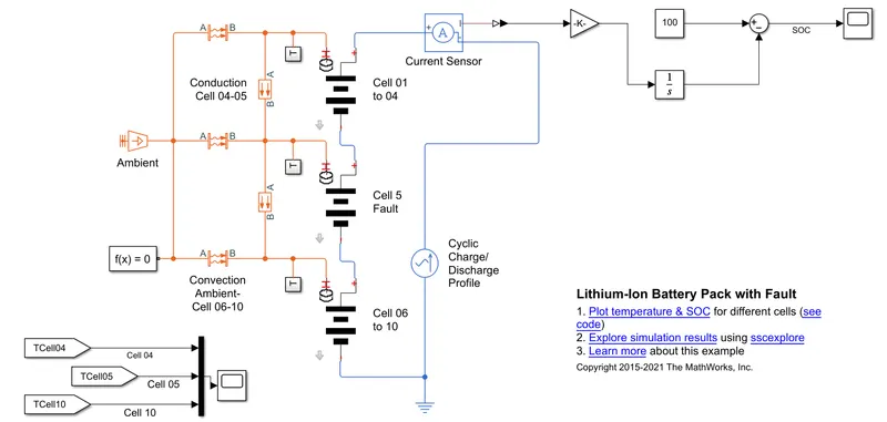
Here I have modified (reduced) the number of cells from 20 lithium-ion cells connected in series to 10 lithium-ion cells connected in series. Cell number 05 has a fault and will be able to discover how can one cell which is connected in series can affect the whole cell if there is no Battery Thermal Management System (BTMS) present along with the battery or with the battery. Single-cell which is connected in series can affect the entire battery pack.
Therefore, it is preferred that the cells be connected in parallel and along with switches to minimize the damage caused to the battery pack capacity as well as to the open-circuit voltage which ultimately results in an increase in the resistance value. Parallelly connected cells result in an increase in current, if any one of the cells connected in parallel goes into a faulty state, then the current can be cut-off, particularly of that parallelly connected cell group can be easy with the help of a fuse, or a switch (we can turn the switch off whenever the cell goes into the faulty state and protect the entire group of cells without affecting the capacity of the battery pack).
Detailed Model explanation with blocks used-
1) Solver configuration-

Solver configuration is used to simulate the model without getting an error, the error may occur because MATLAB uses its default solving configuration for every simulation but in the case of Simulink and Simscape we need to use Solver configuration because Simulink and Simscape both run on a different configuration and by using the Solver configuration block we define the MATLAB system that configuration needs to be calibrated accordingly before simulating the model.
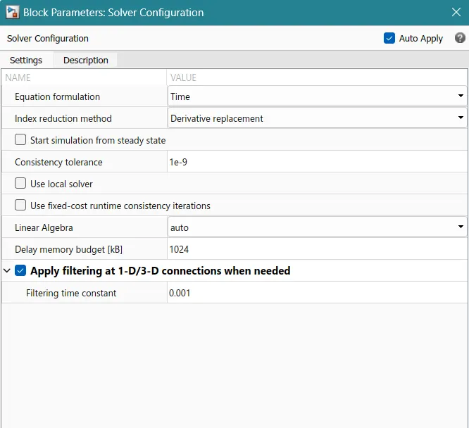
Consistency tolerance is set to 1e-9 which means it is a very small number i.e., 0.000000001, and also, we are filtering time constant by 0.001 seconds.
2) Ambient Temperature -

This block represents an ideal energy source in a thermal network that can maintain a constant absolute temperature at the port regardless of the heat flow rate. The ambient temperature is set to 293.15 k which is nothing but the atmospheric temperature.
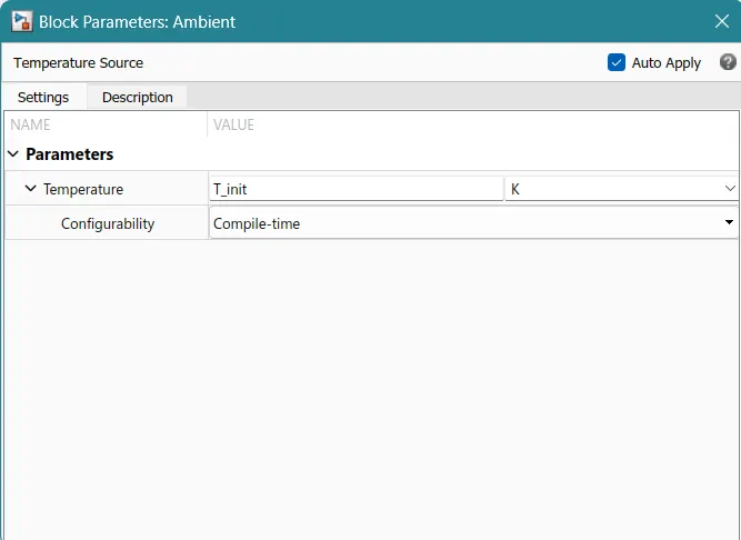
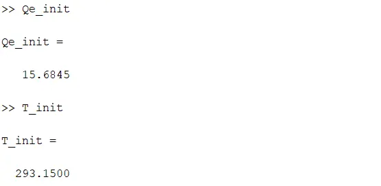
The ambient temperature which carries the value of 293.15 k is stored in the variable called Initial temperature called T_init.
3) Convection Ambient (Heat Transfer block)-
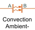
This block models heat transfer in a thermal network by convection due to fluid motion. The rate of heat transfer is proportional to the temperature difference, heat transfer coefficient, and surface area in contact with the fluid.
Convective heat transfer is the transfer of heat between two bodies by currents of moving gas or fluid. In free convection, air or water moves away from the heated body as the warm air or water rises and is replaced by a cooler parcel of air or water. In forced convection, air or water is forcibly moved across the body surface (such as in wind or wind-generated water currents) and efficiently removes heat from the body.
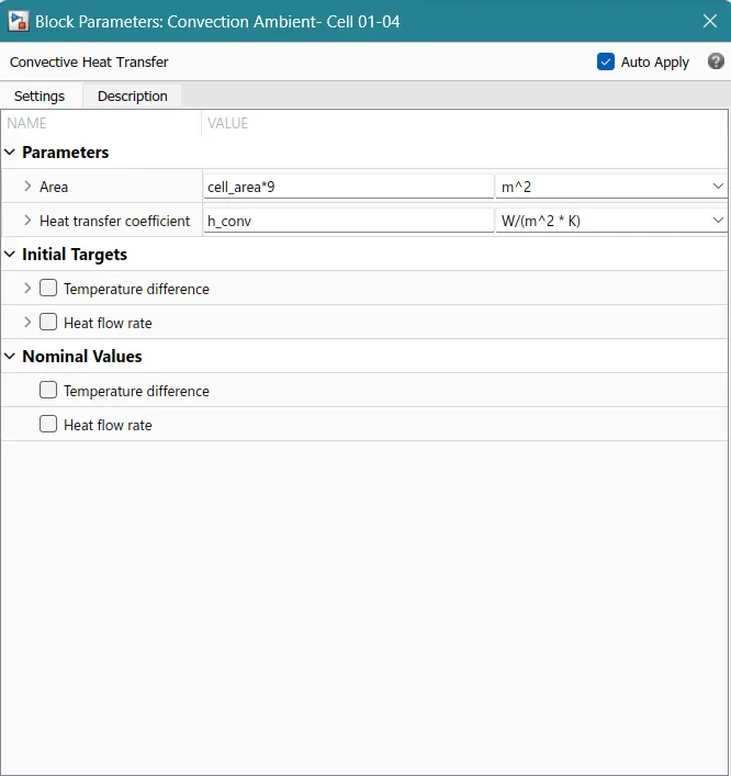
Here the contact surface area is set to 0.1019* 9 m^2. The value 0.1019 is stored in the MATLAB variable called cell_area. From the previous project model, we determined that as the contact surface area increases the heat dissipates quicker, and, as the contact surface area decreases the heat takes time to dissipate as there is less space(area) for heat transfer.
Heat transfer coefficient having a value of 5 W/ (m^2 * k) is stored in the MATLAB variable, as convection heat called h_conv.
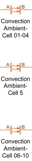
3 convection ambient sources are used here for different configured cells
4) Conduction Cell-
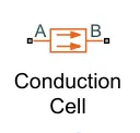
This block models heat transfer in a thermal network by conduction through a layer of material. The rate of heat transfer is governed by Fourier's law and is proportional to the temperature difference, material thermal conductivity, area normal to the heat flow direction, and inversely proportional to the layer thickness.
In conduction, heat transfer occurs between objects by direct contact. Heat transfer takes place due to the difference in temperature. Heat transfer in conduction is slow.
The thermal conductivity of a material is a measure of its ability to conduct heat. It is commonly denoted by,  , or
, or  .
.
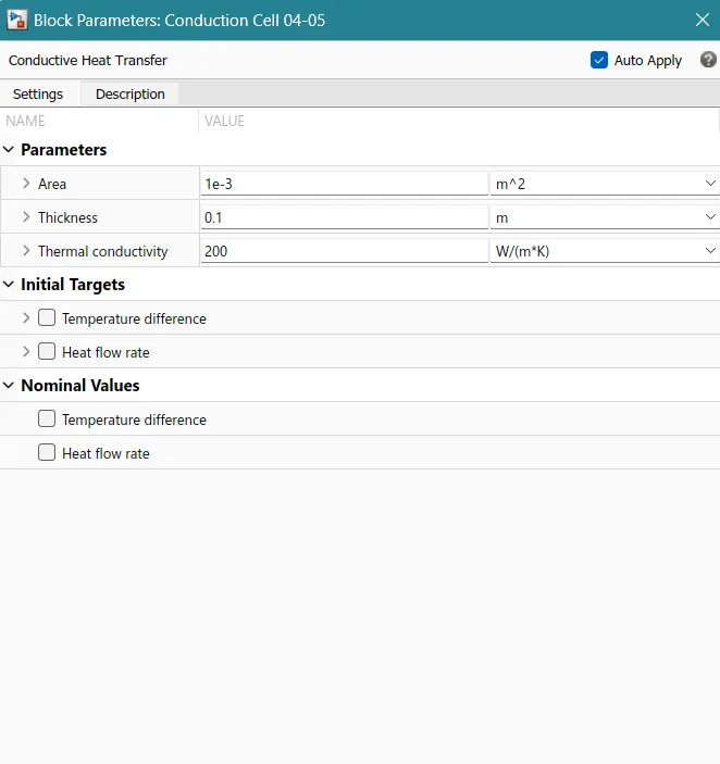
Here we have to set the parameters such as contact surface area for heat dissipation (which is set to 0.001 m^2), the thickness of the cell material (which is set to 0.1 m) as well as the heat conductivity or the thermal conductivity of the material through which the heat is dissipated (which is set to 200 W/(m*k)).
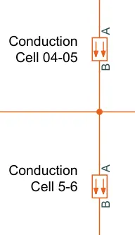
2 such conduction cells are used here for different configured cells
5) Temperature Subsystem Block -

Inside the T subsystem, we have, Temperature sensor block -

This block measures temperature in a thermal network. There is no heat flow through the sensor. The physical signal port T reports the temperature difference across the sensor. The measurement is positive when the temperature at port A is greater than the temperature at port B.
We are giving the input of temperature, T (Which comes from the Thermal Model) to port A, and port B is connected to the thermal reference. Through port T, we get the cell temperature and we can observe the changes occurring in the cell behavior.
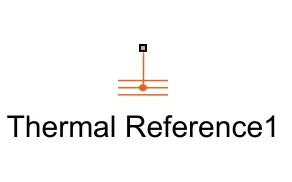
This block represents a reference point in a thermal network where the temperature is equal to absolute zero. Acts as a ground reference for thermal inputs.
Three similar Temperature subsystems are connected in order to observe the temperature changes occurring in the cell behavior.
6) Cell Block-
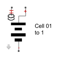
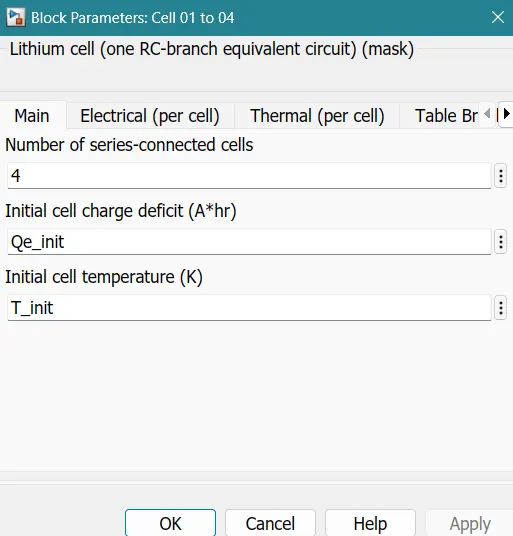
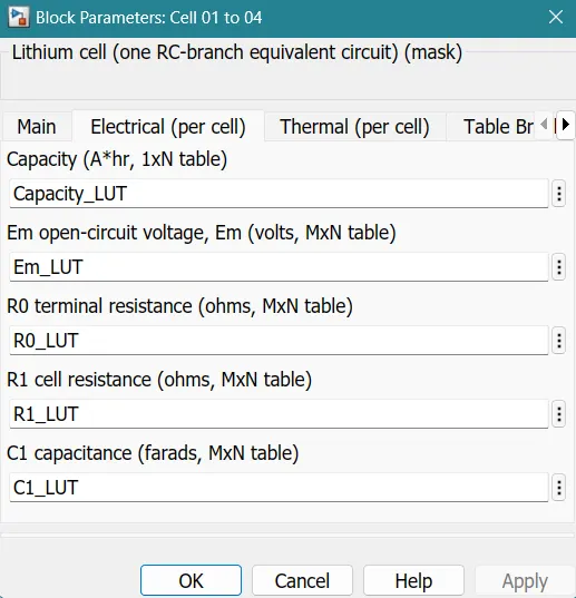
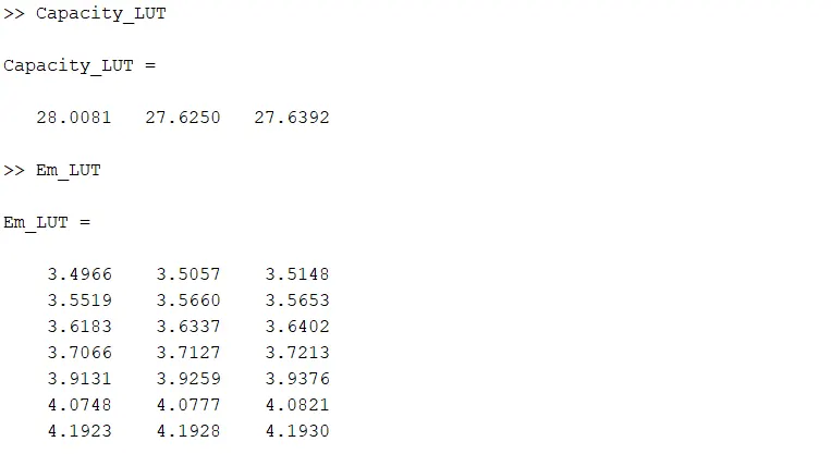
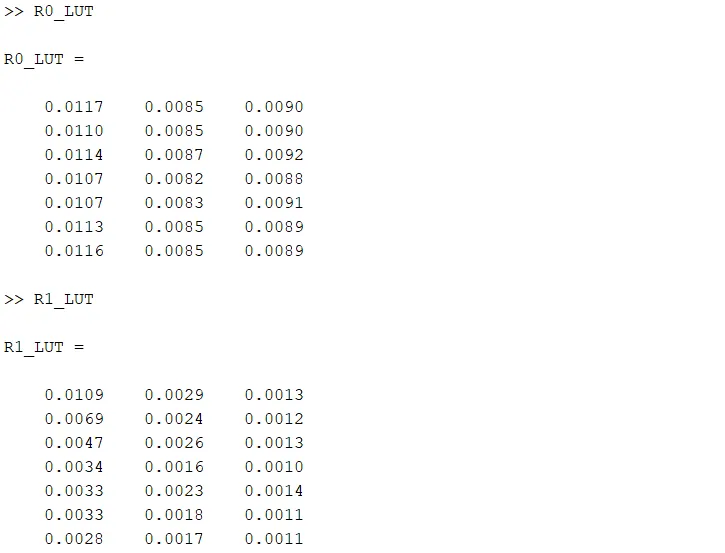
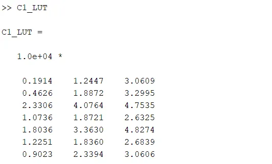
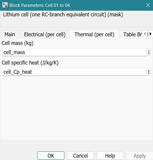
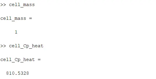
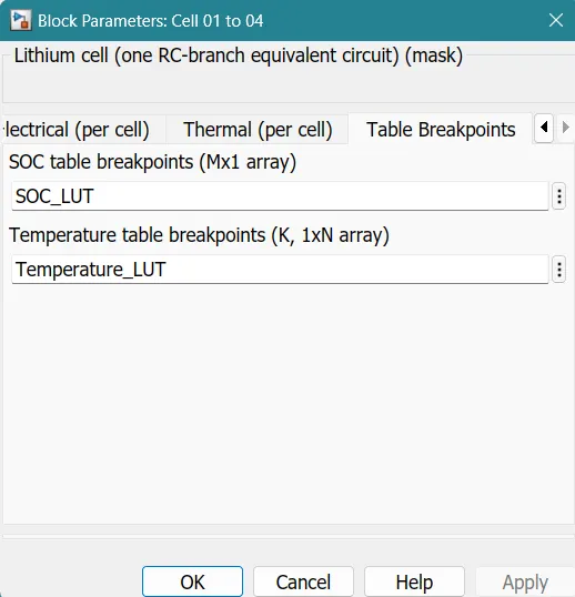
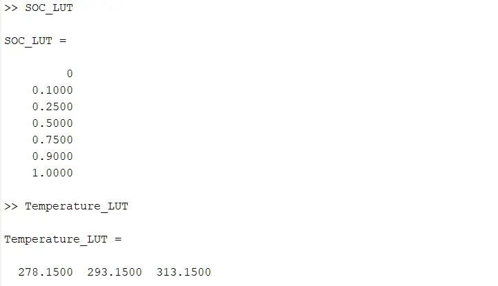
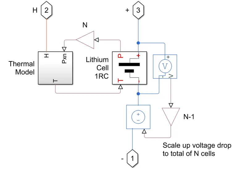
This block represents cell number 1, cell number 2, cell number 3, and cell number 4 connected in a series combination. The cell is nothing but Lithium-Cell. We can define the cell parameters such as electrical properties (Capacity, Open-circuit voltage, Terminal Resistance, Cell Resistance, Capacitance), thermal properties (Mass and Specific heat), and SOC, Temperature breakpoints.
Thermal Model Subsystem:
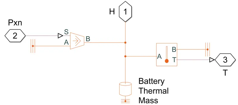
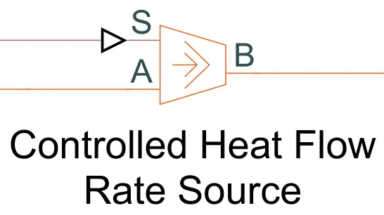
This block represents an ideal energy source in a thermal network that can maintain a controlled heat flow rate regardless of the temperature difference. The heat flow rate is set by the physical signal port S. A positive heat flow rate flows from port A to port B.
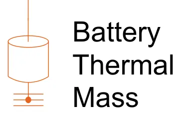
This block models internal energy storage in a thermal network. The rate of temperature increase is proportional to the heat flow rate into the material and inversely proportional to the mass and specific heat of the material.
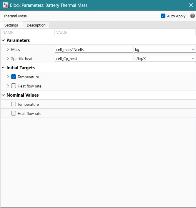
Here, the Entire mass is calculated to be cell mass * a number of cells, in our case it is cell_mass*Ncells.
Lithium-Cell Subsystem:
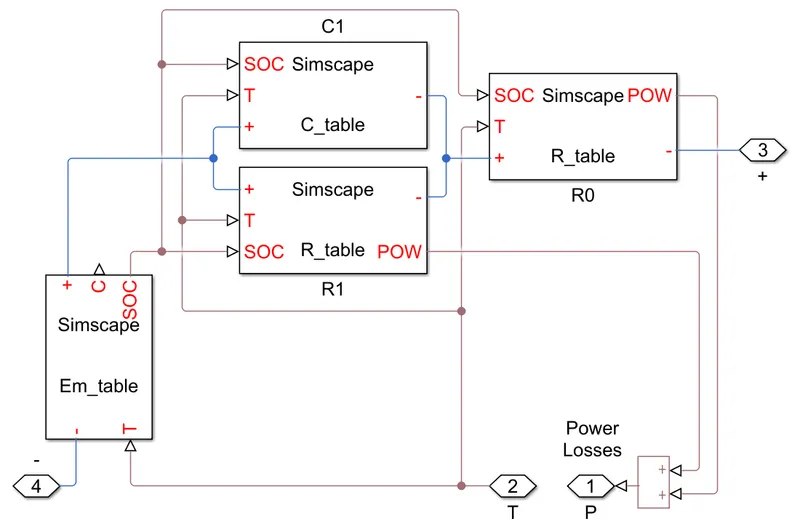
7) C-Table -
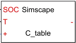
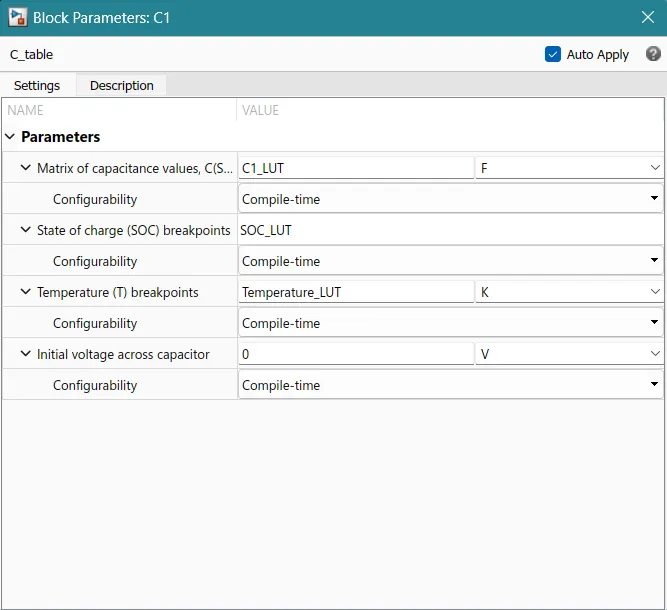
Models a capacitor where the capacitance value (C) depends on an external physical signal inputs SOC and T. It is assumed that the capacitance value is slowly varying with time, and hence the equation i = C*dv/dt holds.
Parameters can be defined in the c-tables such as,
8) Cyclic Charge/Discharge Profile-
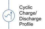
The ideal AC current source maintains the sinusoidal current through it, independent of the voltage across its terminals. The output current is defined by I = I0 * sin (2*pi*f*t + PHI), where I0 is the peak amplitude, f is the frequency in Hz, and PHI is the phase shift in radians.
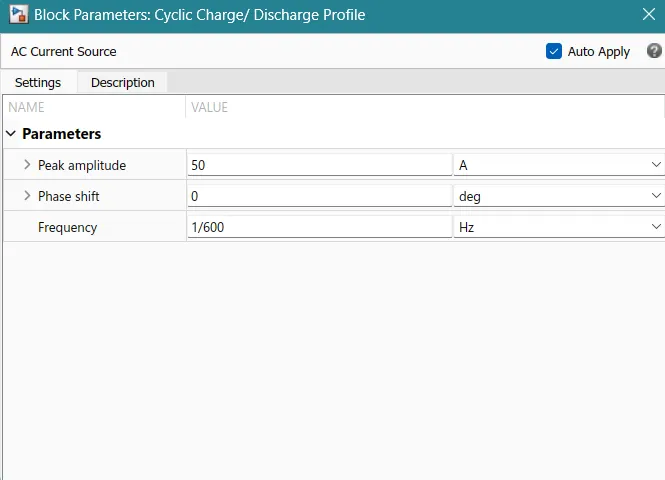
The peak amplitude of the charge and discharge current is set to 50 A, where there are no phase shifts (set to 0 degree), and the frequency is set to 1/600 Hertz.
9) Current Sensor-
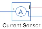
The block represents an ideal current sensor, that is, a device that converts current measured in any electrical branch into a physical signal proportional to the current.
Connections + and - are conserving electrical ports through which the sensor is inserted into the circuit. Connection I is a physical signal port that outputs the current value.
The positive terminal is connected to the far most positive terminal of the cells and the negative terminal is connected to the far most negative terminal of the cells.
10) SOC calculation-
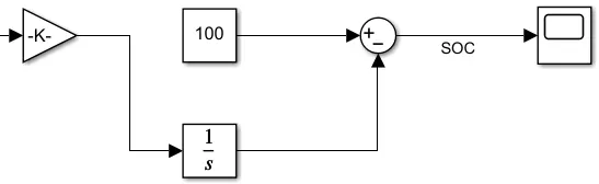
For soc calculation, we have integrated the time constant and subtracted it from 100.
Observations and Results -
We will conduct some tests and observe the changes accordingly, Test sequence is given below,

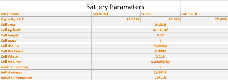
Plots -
Test 1:
a. Cell temperature curve:

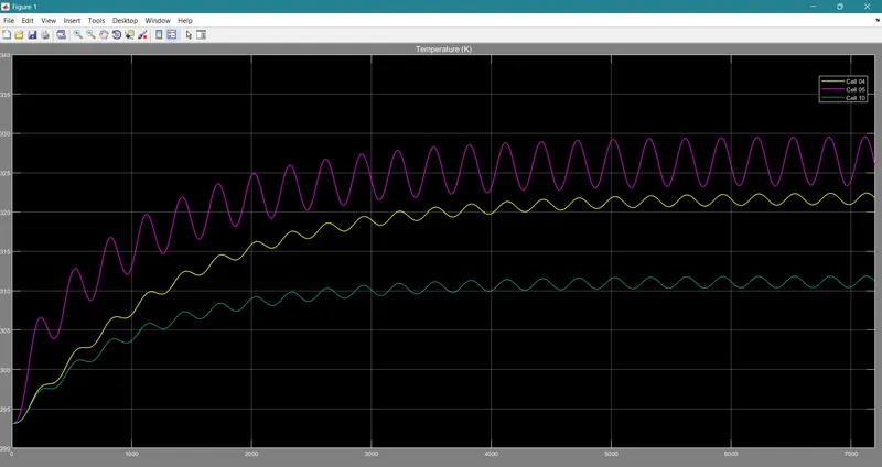
Every cell is given the same initial temperature value of 293.15 k, the temperature for cells 01-04 (yellow line) raises from 294 k to 322 k, whereas, cell number 5 (Purple line) having a faulty state oscillates more as compared to cell numbers 01-04 and reaches a temperature of 326 k, and the temperature for cells 06-10 (Blue line) seems to be more stable than other cells, this is because the contact surface area for cells 06-10 is more than that of cell 01-04 and cell 05, allowing heat to dissipate quickly and easily, resulting the temperature to be the lowest of all.
b. SOC curve:
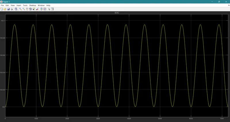
For the ambient temperature of 293.15 k, the state of charge (SOC) curve for each cell reaches from 100 to 100.09, because of the faulty cell which is connected in a series combination.
c. Conduction cell 04-05:
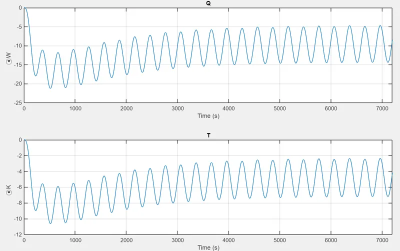
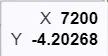
Here, we are plotting the heat flow (unit = W) and temperature (unit = k) with respect to time. We can observe that the waveform drops down as soon as the simulation starts and it enters into a negative amplitude zone within 20 seconds of the simulation. It follows a high amplitude sinusoidal wave throughout the simulation and ends up having a heat transfer coefficient of -8.40 W/m^2*k and a thermal conductivity of -4.20 W/ m*k
heat transfer coefficient:
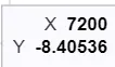
thermal conductivity:
d. Conduction cell 05-06:
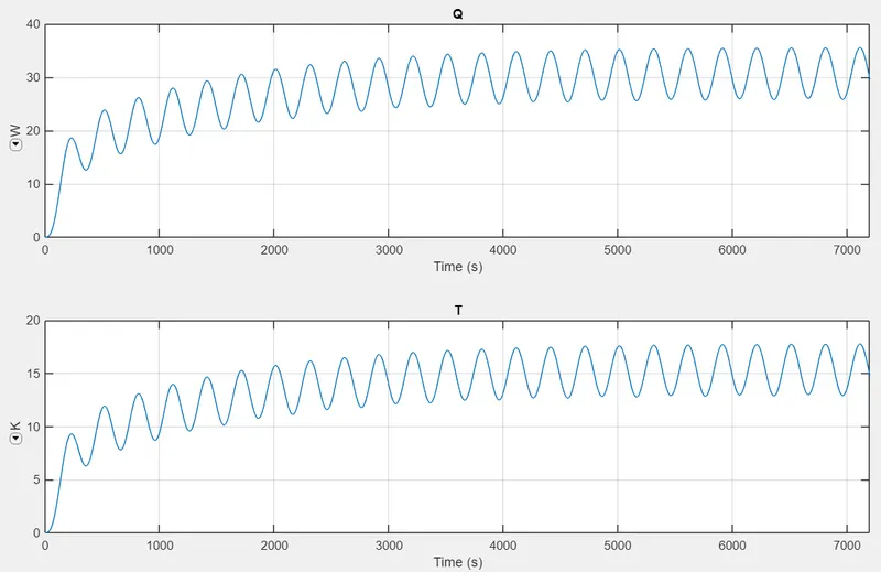
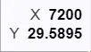
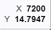
Here, we are plotting the heat flow (unit = W) and temperature (unit = k) with respect to time. We can observe that the waveform spikes up as soon as the simulation starts and it enters into a positive amplitude zone within 20 seconds of the simulation. It follows a high amplitude sinusoidal wave throughout the simulation and ends up having a heat transfer coefficient of 29.5895 W/m^2*k and thermal conductivity of 14.7947 W/ m*k
heat transfer coefficient:
thermal conductivity:
e. Convection cell 01-04:
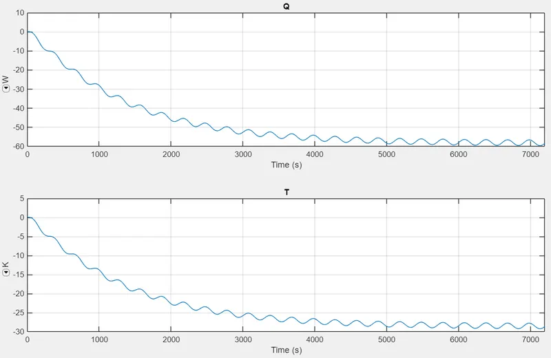
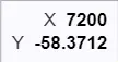
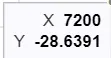
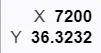
For convection cells 01-04 the oscillations are pretty low and drop into the negative zone at the end of the simulation, i.e., after 7200 seconds. The heat transfer coefficient is -58.3712 W/(m2K) and the Thermal conductivity is -28.6391 W/m K.
The heat transfer coefficient:
Thermal conductivity:
f. Convection cell 05:
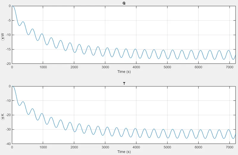
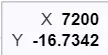
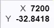
For convection cell 5 it starts from 0 and falls into the negative amplitude zone, the oscillation having high amplitude because of the faulty cell at the end of the simulation i.e., after 7200 seconds. The heat transfer coefficient is -16.7342 W/(m2K) and the Thermal conductivity is -32.8418 W/m K.
The heat transfer coefficient:
Thermal conductivity:
g. Convection cell 06-10:
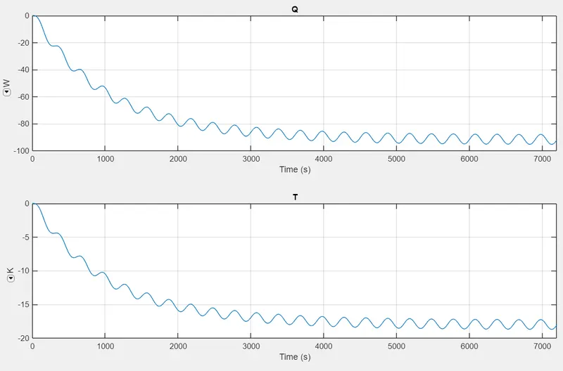
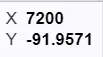
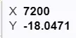
Similar to convection cells 01-04, the pattern of oscillation is almost similar but with a little more amplitude. The faulty cell has affected the following cells and ended up having a heat transfer coefficient is -19.9571 W/(m2K) and a Thermal conductivity is -18.0471 W/m K.
Heat transfer coefficient:
Thermal conductivity:
h. Cyclic Charge/Discharge profiles:
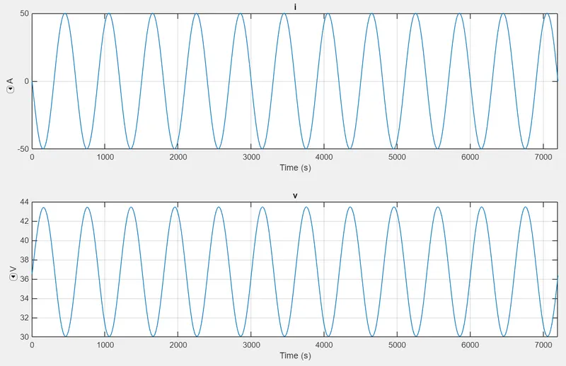
From the cyclic charge and discharge rate graph, we can observe the current and voltage curves with respect to time, the amplitude of the curve is pretty high, where the current oscillates from -50 A to 50 A and the voltage oscillates from 30 V to 43 V (approximately).
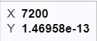
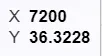
After 7200 seconds of simulation,
Current:
Voltage:
Test 2:

a. Cell temperature curve:
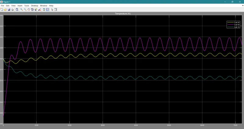
Cell 01-04 and cell 06-10 both groups start from the temperature of 320 k, whereas cell 05 starts from 293.15 k which is the ambient temperature itself. The temperature for cells 01-04 (yellow line) raises from 320 k to 322.5 k, whereas, cell number 5 (Purple line) has a faulty state that oscillates more as compared to cell numbers 01-04 and reaches a temperature of 326 k from 293.15 k, and the temperature for cells 06-10 (Blue line) seems to go down on temperature, this is because the contact surface area for cells 06-10 is more than that of cell 01-04 and cell 05, allowing heat to dissipate quickly and easily, resulting the temperature to be the lowest of all, falling from 320 k to 311 k.
b. SOC curve:
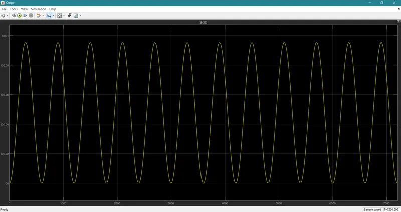
For the ambient temperature of 320 k set to cell 01-04 and cell 06-10, as well as cell 05 sets to 293.15 k, the state of charge (SOC) curve for each cell, reaches from 100 to 100.09, because of the faulty cell which is connected in a series combination.
c. Conduction cell 04-05:
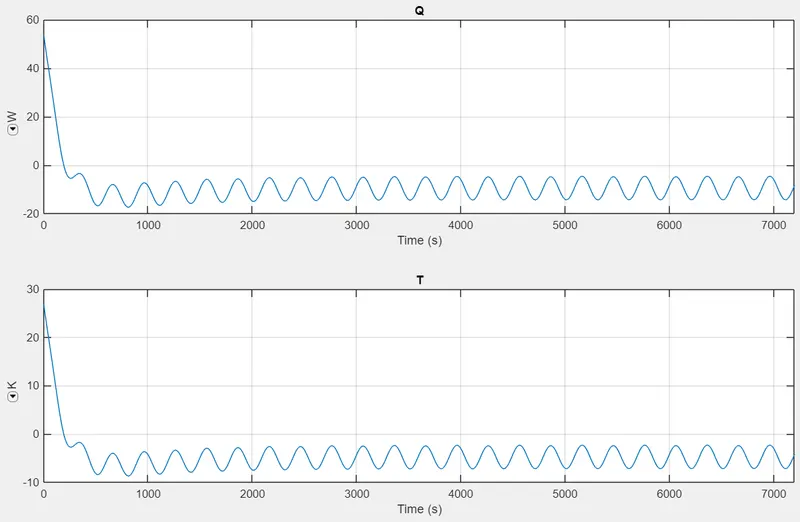
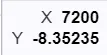
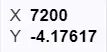
Here, we are plotting the heat flow (unit = W) and temperature (unit = k) with respect to time. We can observe that the waveform drops down as soon as the simulation starts and it enters into a negative amplitude zone within 20 seconds of the simulation. It follows a high amplitude sinusoidal wave throughout the simulation and ends up having a heat transfer coefficient of -8.35235 W/m^2*k and a thermal conductivity of -4.17617 W/ m*k
heat transfer coefficient:
thermal conductivity:
d. Conduction cell 05-06:
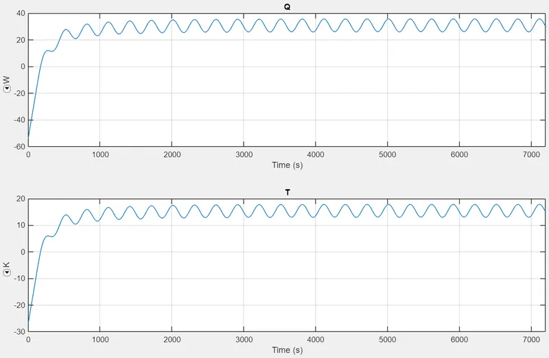
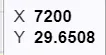
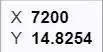
Here, we are plotting the heat flow (unit = W) and temperature (unit = k) with respect to time. We can observe that the waveform spikes up as soon as the simulation starts and it enters into a positive amplitude zone within 20 seconds of the simulation. It follows a high amplitude sinusoidal wave throughout the simulation and ends up having a heat transfer coefficient of 29.6508 W/m^2*k and thermal conductivity of 14.8254 W/ m*k
heat transfer coefficient:
thermal conductivity:
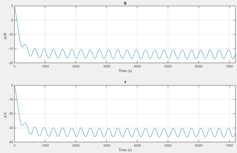
e. Convection cell 01-04:
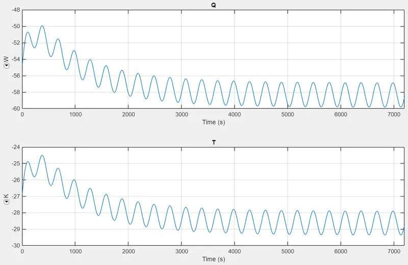
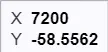
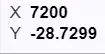
For convection cells 01-04 the oscillations are pretty high and start off from the negative zone. The heat transfer coefficient is -58.5562 W/(m2K) and the Thermal conductivity is -28.7299 W/m K.
The heat transfer coefficient:
Thermal conductivity:
f. Convection cell 05:
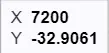
For convection cell 5 it starts from 0 and falls into the negative amplitude zone, the oscillation having high amplitude because of the faulty cell at the end of the simulation i.e., after 7200 seconds. The heat transfer coefficient is -16.767 W/(m2K) and the Thermal conductivity is -32.9061 W/m K.
The heat transfer coefficient:

Thermal conductivity:
g. Convection cell 06-10:
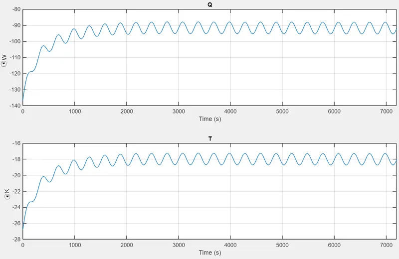
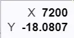
Similar to convection cells 01-04, the pattern of oscillation is almost similar but with a little fewer amplitude. The faulty cell has affected the following cells and ended up having a heat transfer coefficient is -92.1284 W/(m2K) and a Thermal conductivity is -18.0807 W/m K.
Heat transfer coefficient:
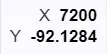
Thermal conductivity:
h. Cyclic Charge/Discharge profiles:
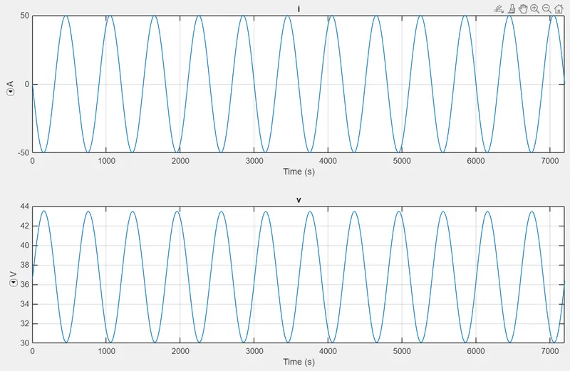
From the cyclic charge and discharge rate graph, we can observe the current and voltage curves with respect to time, the amplitude of the curve is pretty high, where the current oscillates from -50 A to 50 A and the voltage oscillates from 30 V to 43 V (approximately).
After 7200 seconds of simulation,
Current:
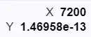
Voltage:

Test 3:

a. Cell temperature curve:
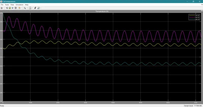
Cell 01-04 starts from the temperature of 320 k, cell 06-10 starts from the temperature of 330 k, whereas cell 05 starts from 340 k. The temperature for cells 01-04 (yellow line) raises from 320 k to 322.5 k, whereas, cell number 5 (Purple line) has a faulty state that oscillates more as compared to cell numbers 01-04 and drops to the temperature of 326 k from 330 k, and the temperature for cells 06-10 (Blue line) seems to go down on temperature, this is because the contact surface area for cells 06-10 is more than that of cell 01-04 and cell 05, allowing heat to dissipate quickly and easily, resulting the temperature to be the lowest of all, falling from 340 k to 311 k.
b. SOC curve:
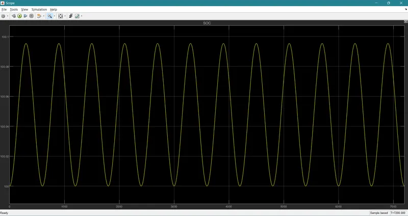
For the increasing range of temperatures for cells 01-04, cell 05, and cell06-10, the state of charge (SOC) curve for each cell reaches from 100 to 100.09, because of the faulty cell which is connected in a series combination.
c. Conduction cell 04-05:
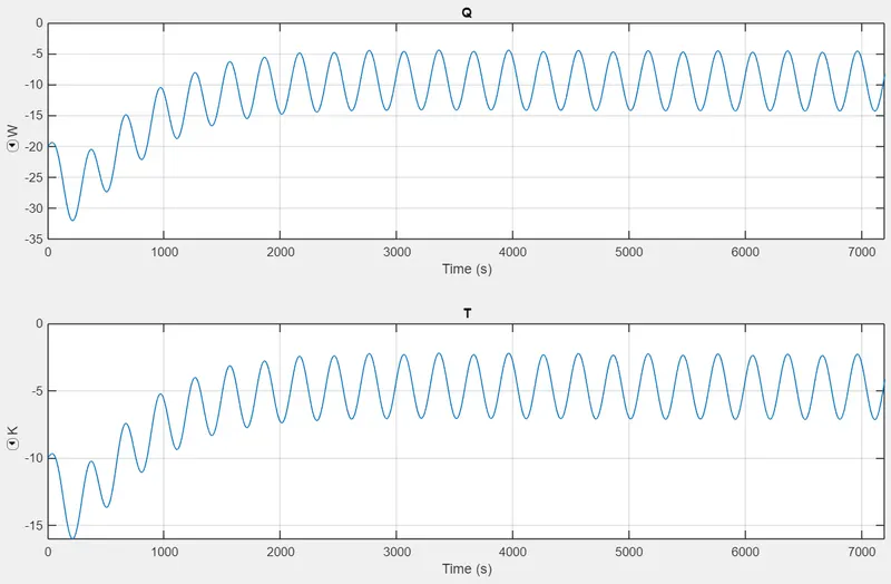
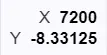
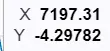
Here, we are plotting the heat flow (unit = W) and temperature (unit = k) with respect to time. We can observe that the waveform drops down as soon as the simulation starts and it enters into a negative amplitude zone within 20 seconds of the simulation followed by which it tries to enter into the positive amplitude zone slowly. It follows a high amplitude sinusoidal wave throughout the simulation and ends up having a heat transfer coefficient of -8.33125 W/m^2*k and a thermal conductivity of -4.29782 W/ m*k
heat transfer coefficient:
thermal conductivity:
d. Conduction cell 05-06:
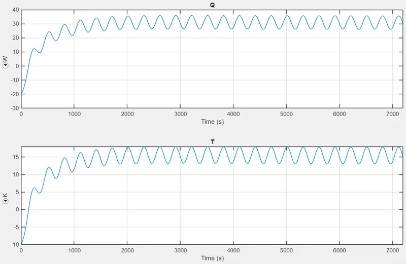
Here, we are plotting the heat flow (unit = W) and temperature (unit = k) with respect to time. We can observe that the waveform spikes up as soon as the simulation starts and it enters into a positive amplitude zone within 20 seconds of the simulation. It follows a high amplitude sinusoidal wave throughout the simulation and ends up having a heat transfer coefficient of 29.6764 W/m^2*k and thermal conductivity of 14.8382 W/ m*k
heat transfer coefficient:

thermal conductivity:

e. Convection cell 01-04:
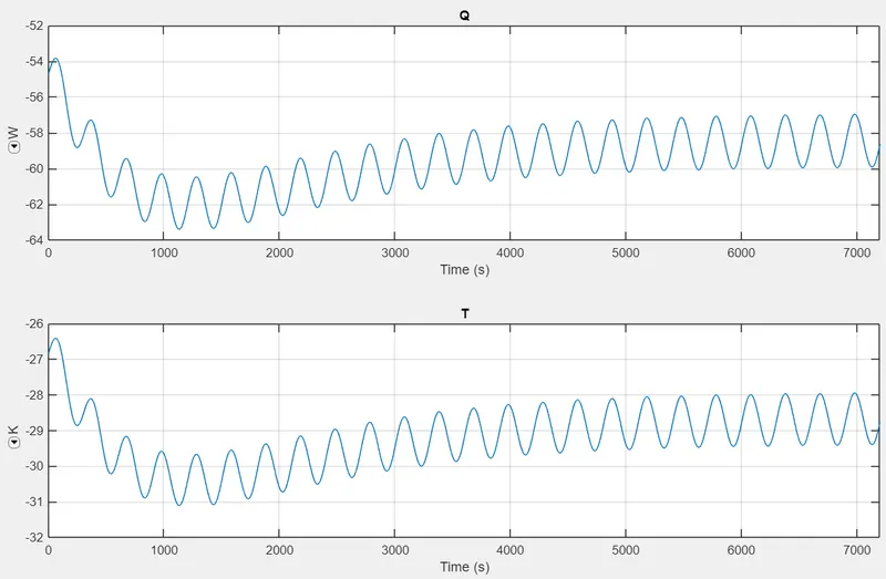
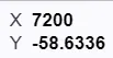
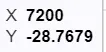
For convection cells 01-04 the oscillations are pretty low and drop into the negative zone at the end of the simulation, i.e., after 7200 seconds. The heat transfer coefficient is -58.6336 W/(m2K) and the Thermal conductivity is -28.7679 W/m K.
The heat transfer coefficient:
Thermal conductivity:
f. Convection cell 05:
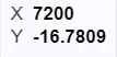
For convection cell 5 it starts from 0 and falls into the negative amplitude zone, the oscillation having high amplitude because of the faulty cell at the end of the simulation i.e., after 7200 seconds. The heat transfer coefficient is -16.7809 W/(m2K) and the Thermal conductivity is -32.9335 W/m K.
The heat transfer coefficient:
Thermal conductivity:

g. Convection cell 06-10:
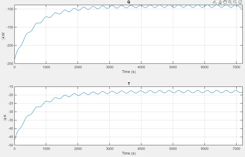
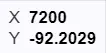
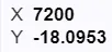
With a fewer (damped) amplitude, cells 06-10 move towards the positive amplitude zone from the negative amplitude zone. The faulty cell has affected the following cells and ended up having a heat transfer coefficient is -92.2029 W/(m2K) and a Thermal conductivity is -18.0853 W/m K.
Heat transfer coefficient:
Thermal conductivity:
h. Cyclic Charge/Discharge profiles:
From the cyclic charge and discharge rate graph, we can observe the current and voltage curves with respect to time, the amplitude of the curve is pretty high, where the current oscillates from -50 A to 50 A and the voltage oscillates from 30 V to 43 V (approximately).
After 7200 seconds of simulation,
Current:

Voltage:

Test 4:

a. Cell temperature curve:
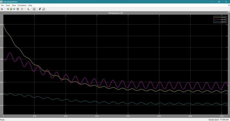
Cell 01-04 starts from a temperature of 380 k, cell 06-10 starts from a temperature of 320 k, whereas cell 05 starts from 350 k. The temperature for cells 01-04 (yellow line) drops from 380 k to 322.5 k, whereas cell number 5 (Purple line) has a faulty state that oscillates more as compared to cell numbers 01-04 and drops to the temperature of 350 k from 325 k, and the temperature for cells 06-10 (Blue line) seems to go down on temperature, this is because the contact surface area for cells 06-10 is more than that of cell 01-04 and cell 05, allowing heat to dissipate quickly and easily, resulting the temperature to be the lowest of all, falling from 320 k to 311 k.
b. SOC curve:
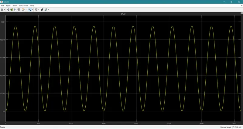
For the ambient temperature of 293.15 k, the state of charge (SOC) curve for each cell reaches from 100 to 100.09, because of the faulty cell which is connected in a series combination.
c. Conduction cell 04-05:
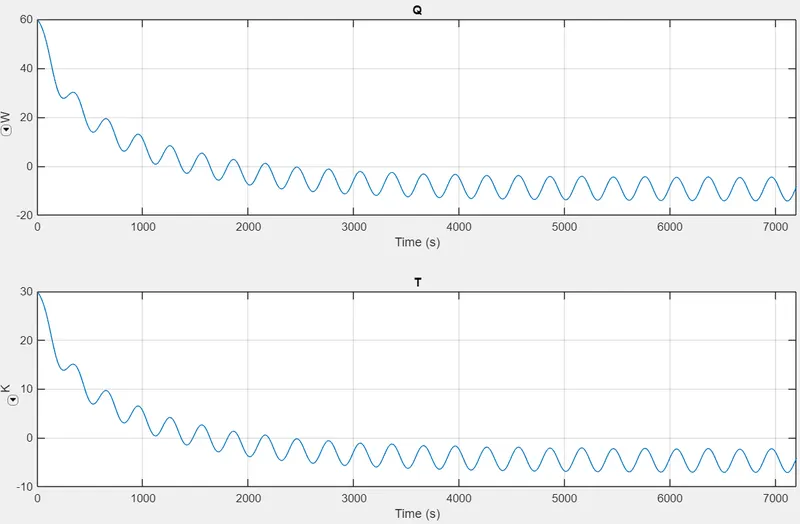
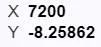
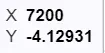
Here, we are plotting the heat flow (unit = W) and temperature (unit = k) with respect to time. We can observe that the waveform drops down as soon as the simulation starts and it enters into a negative amplitude zone within 20 seconds of the simulation. It follows a high amplitude sinusoidal wave throughout the simulation and ends up having a heat transfer coefficient of -8.25862 W/m^2*k and a thermal conductivity of -4.12931 W/ m*k
heat transfer coefficient:
thermal conductivity:
d. Conduction cell 05-06:
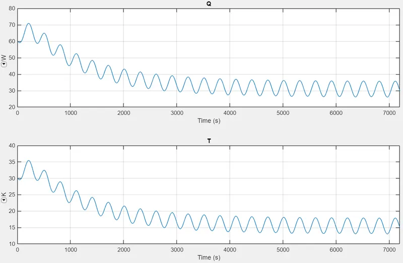
Here, we are plotting the heat flow (unit = W) and temperature (unit = k) with respect to time. We can observe that the waveform drops down after some time of simulation and it stays in a positive amplitude zone. It follows a high amplitude sinusoidal wave throughout the simulation and ends up having a heat transfer coefficient of 29.7624 W/m^2*k and thermal conductivity of 14.7947 W/ m*k
heat transfer coefficient:

thermal conductivity:
e. Convection cell 01-04:
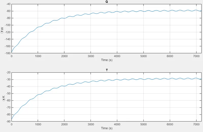
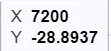
For convection cells 01-04 the oscillations are pretty low and raises up from the negative zone at the end of the simulation, i.e., after 7200 seconds. The heat transfer coefficient is -58.89 W/(m2K) and the Thermal conductivity is -28.8937 W/m K.
The heat transfer coefficient:

Thermal conductivity:
f. Convection cell 05:
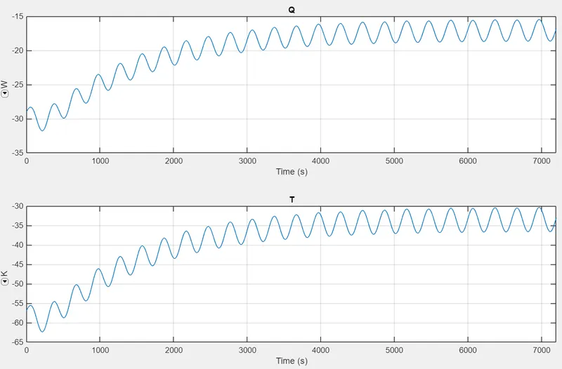
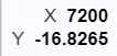
For convection cell 5 it starts from 0 and raise from the negative amplitude zone towards the positive amplitude zone, the oscillation having high amplitude because of the faulty cell at the end of the simulation i.e., after 7200 seconds. The heat transfer coefficient is -16.8265 W/(m2K) and the Thermal conductivity is -33.023 W/m K.
The heat transfer coefficient:
Thermal conductivity:

g. Convection cell 06-10:
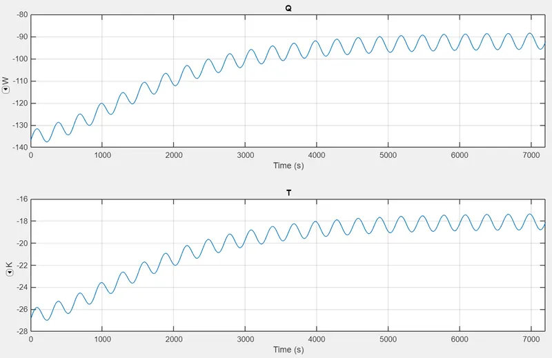
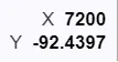
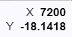
Similar to convection cells 01-04, the pattern of oscillation is almost similar but with a little more amplitude. The faulty cell has affected the following cells and ended up having a heat transfer coefficient is -92.4397 W/(m2K) and a Thermal conductivity is -18.1418 W/m K.
Heat transfer coefficient:
Thermal conductivity:
h. Cyclic Charge/Discharge profiles:
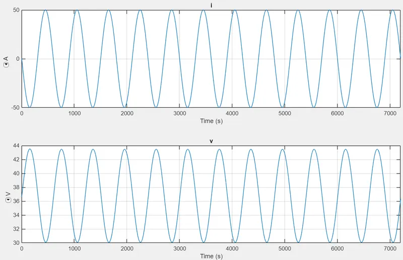
From the cyclic charge and discharge rate graph, we can observe the current and voltage curves with respect to time, the amplitude of the curve is pretty high, where the current oscillates from -50 A to 50 A and the voltage oscillates from 30 V to 43 V (approximately).
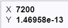
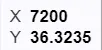
After 7200 seconds of simulation,
Current:
Voltage:
Test 5:

a. Cell temperature curve:
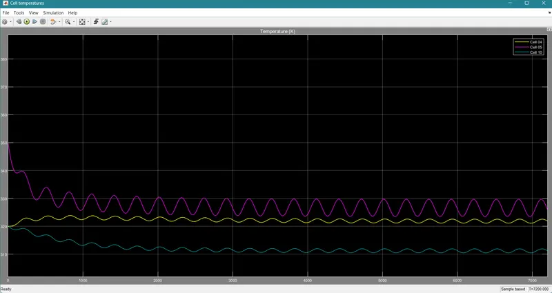
Cell 01-04 and cell 06-10 are given the same initial temperature value of 320k, while cell 5 is given the initial temperature of 350 k, the temperature for cells 01-04 (yellow line) raises from 320 k to 322 k, whereas, cell number 5 (Purple line) has a faulty state oscillates more as compared to cell numbers 01-04 and drops down to the temperature of 326 k, and the temperature for cells 06-10 (Blue line) seems to be similar to that of cell 01-04, but resulting the temperature to be the lowest of all which is at 311 k, this is because the contact surface area for cells 06-10 is more than that of cell 01-04 and cell 05, allowing heat to dissipate quickly and easily.
b. SOC curve:
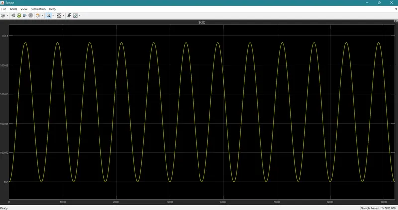
For the ambient temperature of 293.15 k, the state of charge (SOC) curve for each cell reaches from 100 to 100.09, because of the faulty cell which is connected in a series combination.
c. Conduction cell 04-05:
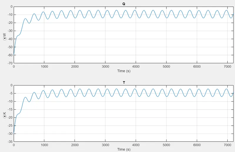
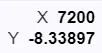
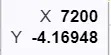
Here, we are plotting the heat flow (unit = W) and temperature (unit = k) with respect to time. We can observe that the waveform spikes up as soon as the simulation starts and it enters into a positive amplitude zone within 10 seconds of the simulation. It follows a high amplitude sinusoidal wave throughout the simulation and ends up having a heat transfer coefficient of -8.33897 W/m^2*k and a thermal conductivity of -4.16948 W/ m*k
heat transfer coefficient:
thermal conductivity:
d. Conduction cell 05-06:
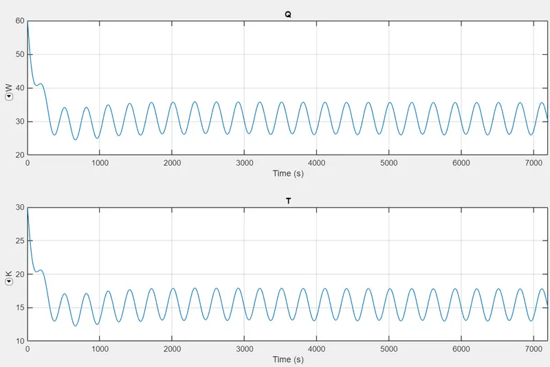
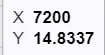
Here, we are plotting the heat flow (unit = W) and temperature (unit = k) with respect to time. We can observe that the waveform drops down as soon as the simulation starts and stays in the positive amplitude zone throughout the simulation. It follows a high amplitude sinusoidal wave throughout the simulation and ends up having a heat transfer coefficient of 29.6674 W/m^2*k and thermal conductivity of 14.8337 W/ m*k
heat transfer coefficient:
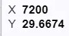
thermal conductivity:
e. Convection cell 01-04:
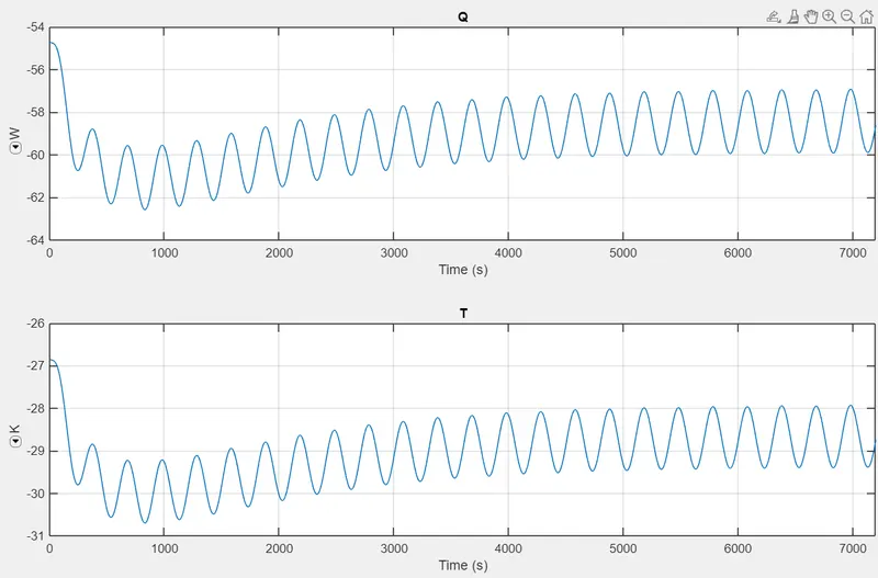
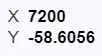
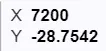
For convection cells 01-04 the oscillations are pretty high and drop into the negative zone at the end of the simulation, i.e., after 7200 seconds. The heat transfer coefficient is -58.6056 W/(m2K) and the Thermal conductivity is -28.7542 W/m K.
The heat transfer coefficient:
Thermal conductivity:
f. Convection cell 05:
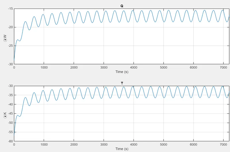
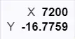
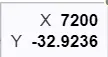
For convection cell 5 it starts from 0 seconds and tries to stabilize it but is still in the negative amplitude zone, the oscillation having high amplitude because of the faulty cell at the end of the simulation i.e., after 7200 seconds. The heat transfer coefficient is -16.7759 W/(m2K) and the Thermal conductivity is -32.9236 W/m K.
The heat transfer coefficient:
Thermal conductivity:
g. Convection cell 06-10:
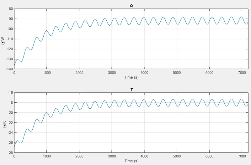
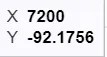
With a little more amplitude cell 06-10 tries to stabilize themselves but is still in the negative amplitude zone. The faulty cell has affected the following cells and ended up having a heat transfer coefficient is -92.1756 W/(m2K) and a Thermal conductivity is -18.09 W/m K.
Heat transfer coefficient:
Thermal conductivity:

h. Cyclic Charge/Discharge profiles:
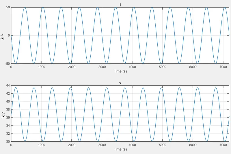
From the cyclic charge and discharge rate graph, we can observe the current and voltage curves with respect to time, the amplitude of the curve is pretty high, where the current oscillates from -50 A to 50 A and the voltage oscillates from 30 V to 43 V (approximately).
After 7200 seconds of simulation,
Current:
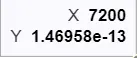
Voltage:
Conclusion:
1) SOC remains constant throughout the simulation.
2) Cell temperatures are more stable when the faulty cell temperature is higher than the other 2 groups of cell temperature.
3) Cell 06-10 is tempered (Unstable) because of the fact that cell 05 is in a faulty state.
2) Heat flow through conduction and convection changes as there are changes in temperature.
Bibliography -
3) Conduction Mode of Heat Transfer
Drive link - https://drive.google.com/drive/folders/1RJe-vQKgmvXQBgEAIW5TVLxiet8yAR_C?usp=sharing